indhub commented on a change in pull request #10959: [MXNET-423] Gluon Model
Zoo Pre Trained Model tutorial
URL: https://github.com/apache/incubator-mxnet/pull/10959#discussion_r189128940
########## File path: docs/tutorials/gluon/pretrained_models.md ########## @@ -0,0 +1,374 @@ + +# Using pre-trained models in MXNet + +In this tutorial we will see how to use multiple pre-trained models with Apache MXNet. First, let's download three image classification models from the Apache MXNet [Gluon model zoo](https://mxnet.incubator.apache.org/api/python/gluon/model_zoo.html). +* **DenseNet-121** ([research paper](https://arxiv.org/abs/1608.06993)), improved state of the art on [ImageNet dataset](http://image-net.org/challenges/LSVRC) in 2016. +* **MobileNet** ([research paper](https://arxiv.org/abs/1704.04861)), MobileNets are based on a streamlined architecture that uses depth-wise separable convolutions to build light weight deep neural networks, suitable for mobile applications. +* **ResNet-18** ([research paper](https://arxiv.org/abs/1512.03385v1)), the -152 version is the 2015 winner in multiple categories. + +Why would you want to try multiple models? Why not just pick the one with the best accuracy? As we will see later in the tutorial, even though these models have been trained on the same dataset and optimized for maximum accuracy, they do behave slightly differently on specific images. In addition, prediction speed and memory footprints can vary, and that is an important factor for many applications. By trying a few pretrained models, you have an opportunity to find a model that can be a good fit for solving your business problem. + + +```python +import json + +import matplotlib.pyplot as plt +import mxnet as mx +from mxnet import gluon, nd +from mxnet.gluon.model_zoo import vision +import numpy as np +%matplotlib inline +``` + +## Loading the model + +The [Gluon Model Zoo](https://mxnet.incubator.apache.org/api/python/gluon/model_zoo.html) provides a collection of off-the-shelf models. You can get the ImageNet pre-trained model by using `pretrained=True`. +If you want to train on your own classification problem from scratch, you can get an untrained network with a specific number of classes using the `classes` parameter: for example `net = vision.resnet18_v1(classes=10)`. However note that you cannot use the `pretrained` and `classes` parameter at the same time. If you want to use pre-trained weights as initialization of your network except for the last layer, have a look at the last section of this tutorial. + +We can specify the *context* where we want to run the model: the default behavior is to use a CPU context. There are two reasons for this: +* First, this will allow you to test the notebook even if your machine is not equipped with a GPU :) +* Second, we're going to predict a single image and we don't have any specific performance requirements. For production applications where you'd want to predict large batches of images with the best possible throughput, a GPU could definitely be the way to go. +* If you want to use a GPU, make sure you have pip installed the right version of mxnet, or you will get an error when using the `mx.gpu()` context. Refer to the [install instructions](http://mxnet.incubator.apache.org/install/index.html) + + +```python +# We set the context to CPU, you can switch to GPU if you have one and installed a compatible version of MXNet +ctx = mx.cpu() +``` + + +```python +# We can load three the three models +densenet121 = vision.densenet121(pretrained=True, ctx=ctx) +mobileNet = vision.mobilenet0_5(pretrained=True, ctx=ctx) +resnet18 = vision.resnet18_v1(pretrained=True, ctx=ctx) +``` + +We can look at the description of the MobileNet network for example, which has a relatively simple yet deep architecture + + +```python +print(mobileNet) +``` + + MobileNet( + (features): HybridSequential( + (0): Conv2D(3 -> 16, kernel_size=(3, 3), stride=(2, 2), padding=(1, 1), bias=False) + (1): BatchNorm(axis=1, eps=1e-05, momentum=0.9, fix_gamma=False, use_global_stats=False, in_channels=16) + (2): Activation(relu) + (3): Conv2D(1 -> 16, kernel_size=(3, 3), stride=(1, 1), padding=(1, 1), groups=16, bias=False) + (4): BatchNorm(axis=1, eps=1e-05, momentum=0.9, fix_gamma=False, use_global_stats=False, in_channels=16) + (5): Activation(relu) + (6): Conv2D(16 -> 32, kernel_size=(1, 1), stride=(1, 1), bias=False) + (7): BatchNorm(axis=1, eps=1e-05, momentum=0.9, fix_gamma=False, use_global_stats=False, in_channels=32) + (8): Activation(relu) + (9): Conv2D(1 -> 32, kernel_size=(3, 3), stride=(2, 2), padding=(1, 1), groups=32, bias=False) + (10): BatchNorm(axis=1, eps=1e-05, momentum=0.9, fix_gamma=False, use_global_stats=False, in_channels=32) + (11): Activation(relu) + (12): Conv2D(32 -> 64, kernel_size=(1, 1), stride=(1, 1), bias=False) + (13): BatchNorm(axis=1, eps=1e-05, momentum=0.9, fix_gamma=False, use_global_stats=False, in_channels=64) + (14): Activation(relu) + (15): Conv2D(1 -> 64, kernel_size=(3, 3), stride=(1, 1), padding=(1, 1), groups=64, bias=False) + (16): BatchNorm(axis=1, eps=1e-05, momentum=0.9, fix_gamma=False, use_global_stats=False, in_channels=64) + (17): Activation(relu) + (18): Conv2D(64 -> 64, kernel_size=(1, 1), stride=(1, 1), bias=False) + (19): BatchNorm(axis=1, eps=1e-05, momentum=0.9, fix_gamma=False, use_global_stats=False, in_channels=64) + (20): Activation(relu) + (21): Conv2D(1 -> 64, kernel_size=(3, 3), stride=(2, 2), padding=(1, 1), groups=64, bias=False) + (22): BatchNorm(axis=1, eps=1e-05, momentum=0.9, fix_gamma=False, use_global_stats=False, in_channels=64) + (23): Activation(relu) + (24): Conv2D(64 -> 128, kernel_size=(1, 1), stride=(1, 1), bias=False) + (25): BatchNorm(axis=1, eps=1e-05, momentum=0.9, fix_gamma=False, use_global_stats=False, in_channels=128) + (26): Activation(relu) + (27): Conv2D(1 -> 128, kernel_size=(3, 3), stride=(1, 1), padding=(1, 1), groups=128, bias=False) + (28): BatchNorm(axis=1, eps=1e-05, momentum=0.9, fix_gamma=False, use_global_stats=False, in_channels=128) + (29): Activation(relu) + (30): Conv2D(128 -> 128, kernel_size=(1, 1), stride=(1, 1), bias=False) + (31): BatchNorm(axis=1, eps=1e-05, momentum=0.9, fix_gamma=False, use_global_stats=False, in_channels=128) + (32): Activation(relu) + (33): Conv2D(1 -> 128, kernel_size=(3, 3), stride=(2, 2), padding=(1, 1), groups=128, bias=False) + (34): BatchNorm(axis=1, eps=1e-05, momentum=0.9, fix_gamma=False, use_global_stats=False, in_channels=128) + (35): Activation(relu) + (36): Conv2D(128 -> 256, kernel_size=(1, 1), stride=(1, 1), bias=False) + (37): BatchNorm(axis=1, eps=1e-05, momentum=0.9, fix_gamma=False, use_global_stats=False, in_channels=256) + (38): Activation(relu) + (39): Conv2D(1 -> 256, kernel_size=(3, 3), stride=(1, 1), padding=(1, 1), groups=256, bias=False) + (40): BatchNorm(axis=1, eps=1e-05, momentum=0.9, fix_gamma=False, use_global_stats=False, in_channels=256) + (41): Activation(relu) + (42): Conv2D(256 -> 256, kernel_size=(1, 1), stride=(1, 1), bias=False) + (43): BatchNorm(axis=1, eps=1e-05, momentum=0.9, fix_gamma=False, use_global_stats=False, in_channels=256) + (44): Activation(relu) + (45): Conv2D(1 -> 256, kernel_size=(3, 3), stride=(1, 1), padding=(1, 1), groups=256, bias=False) + (46): BatchNorm(axis=1, eps=1e-05, momentum=0.9, fix_gamma=False, use_global_stats=False, in_channels=256) + (47): Activation(relu) + (48): Conv2D(256 -> 256, kernel_size=(1, 1), stride=(1, 1), bias=False) + (49): BatchNorm(axis=1, eps=1e-05, momentum=0.9, fix_gamma=False, use_global_stats=False, in_channels=256) + (50): Activation(relu) + (51): Conv2D(1 -> 256, kernel_size=(3, 3), stride=(1, 1), padding=(1, 1), groups=256, bias=False) + (52): BatchNorm(axis=1, eps=1e-05, momentum=0.9, fix_gamma=False, use_global_stats=False, in_channels=256) + (53): Activation(relu) + (54): Conv2D(256 -> 256, kernel_size=(1, 1), stride=(1, 1), bias=False) + (55): BatchNorm(axis=1, eps=1e-05, momentum=0.9, fix_gamma=False, use_global_stats=False, in_channels=256) + (56): Activation(relu) + (57): Conv2D(1 -> 256, kernel_size=(3, 3), stride=(1, 1), padding=(1, 1), groups=256, bias=False) + (58): BatchNorm(axis=1, eps=1e-05, momentum=0.9, fix_gamma=False, use_global_stats=False, in_channels=256) + (59): Activation(relu) + (60): Conv2D(256 -> 256, kernel_size=(1, 1), stride=(1, 1), bias=False) + (61): BatchNorm(axis=1, eps=1e-05, momentum=0.9, fix_gamma=False, use_global_stats=False, in_channels=256) + (62): Activation(relu) + (63): Conv2D(1 -> 256, kernel_size=(3, 3), stride=(1, 1), padding=(1, 1), groups=256, bias=False) + (64): BatchNorm(axis=1, eps=1e-05, momentum=0.9, fix_gamma=False, use_global_stats=False, in_channels=256) + (65): Activation(relu) + (66): Conv2D(256 -> 256, kernel_size=(1, 1), stride=(1, 1), bias=False) + (67): BatchNorm(axis=1, eps=1e-05, momentum=0.9, fix_gamma=False, use_global_stats=False, in_channels=256) + (68): Activation(relu) + (69): Conv2D(1 -> 256, kernel_size=(3, 3), stride=(2, 2), padding=(1, 1), groups=256, bias=False) + (70): BatchNorm(axis=1, eps=1e-05, momentum=0.9, fix_gamma=False, use_global_stats=False, in_channels=256) + (71): Activation(relu) + (72): Conv2D(256 -> 512, kernel_size=(1, 1), stride=(1, 1), bias=False) + (73): BatchNorm(axis=1, eps=1e-05, momentum=0.9, fix_gamma=False, use_global_stats=False, in_channels=512) + (74): Activation(relu) + (75): Conv2D(1 -> 512, kernel_size=(3, 3), stride=(1, 1), padding=(1, 1), groups=512, bias=False) + (76): BatchNorm(axis=1, eps=1e-05, momentum=0.9, fix_gamma=False, use_global_stats=False, in_channels=512) + (77): Activation(relu) + (78): Conv2D(512 -> 512, kernel_size=(1, 1), stride=(1, 1), bias=False) + (79): BatchNorm(axis=1, eps=1e-05, momentum=0.9, fix_gamma=False, use_global_stats=False, in_channels=512) + (80): Activation(relu) + (81): GlobalAvgPool2D(size=(1, 1), stride=(1, 1), padding=(0, 0), ceil_mode=True) + (82): Flatten + ) + (output): Dense(512 -> 1000, linear) + ) + + +Let's have a closer look at the first convolution layer: + + +```python +print(mobileNet.features[0].params) +``` + +`mobilenet1_conv0_ (Parameter mobilenet1_conv0_weight (shape=(16, 3, 3, 3), dtype=<class 'numpy.float32'>))`<!--notebook-skip-line--> + + +The first layer applies **`16`** different convolutional masks, of size **`InputChannels x 3 x 3`**. For the first convolution, there are **`3`** input channels, the `R`, `G`, `B` channels of the input image. That gives us the weight matrix of shape **`16 x 3 x 3 x 3`**. There is no bias applied in this convolution. + +Let's have a look at the output layer now: + + +```python +print(mobileNet.output) +``` + +`Dense(512 -> 1000, linear)`<!--notebook-skip-line--> + + +Did you notice the shape of layer? The weight matrix is **1000 x 512**. This layer contains 1,000 neurons: each of them will store an activation representative of the probability of the image belonging to a specific category. Each neuron is also fully connected to all 512 neurons in the previous layer. + +OK, enough exploring! Now let's use these models to classify our own images. + +## Loading the data +All three models have been pre-trained on the ImageNet data set which includes over 1.2 million pictures of objects and animals sorted in 1,000 categories. +We get the imageNet list of labels. That way we have the mapping so when the model predicts for example category index `4`, we know it is predicting `hammerhead, hammerhead shark` + + +```python +mx.test_utils.download('https://raw.githubusercontent.com/dmlc/web-data/master/mxnet/doc/tutorials/onnx/image_net_labels.json') +categories = np.array(json.load(open('image_net_labels.json', 'r'))) +print(categories[4]) +``` + +`hammerhead, hammerhead shark` <!--notebook-skip-line--> + + +Get a test image + + +```python +filename = mx.test_utils.download('https://github.com/dmlc/web-data/blob/master/mxnet/doc/tutorials/onnx/images/dog.jpg?raw=true', fname='dog.jpg') +``` + +If you want to use your own image for the test, copy the image to the same folder that contains the notebook and change the following line: + + +```python +filename = 'dog.jpg' +``` + +Load the image as a NDArray + + +```python +image = mx.image.imread(filename) +plt.imshow(image.asnumpy()) +``` + +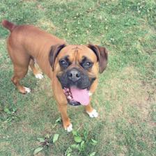 Review comment: <!--notebook-skip-line--> here? ---------------------------------------------------------------- This is an automated message from the Apache Git Service. To respond to the message, please log on GitHub and use the URL above to go to the specific comment. For queries about this service, please contact Infrastructure at: us...@infra.apache.org With regards, Apache Git Services