This is an automated email from the ASF dual-hosted git repository.

xiangfu pushed a commit to branch new-site-dev
in repository https://gitbox.apache.org/repos/asf/pinot-site.git
The following commit(s) were added to refs/heads/new-site-dev by this push:
new 157e9b63 fixed broken images across various older blog posts (#155)
157e9b63 is described below
commit 157e9b63022b40761ff1259c86027c1a3ed86914
Author: James Dilworth <[email protected]>
AuthorDate: Thu Jan 29 23:05:13 2026 -0800
fixed broken images across various older blog posts (#155)
Co-authored-by: James Dilworth <[email protected]>
---
...-Function-For-Time-Series-Datasets-In-Pinot.mdx | 18 +++++++--------
...-11-08-Apache Pinot-How-do-I-see-my-indexes.mdx | 10 ++++-----
.../2022-11-17-Apache Pinot-Inserts-from-SQL.mdx | 10 ++++-----
.../2022-11-22-Apache-Pinot-Timestamp-Indexes.mdx | 12 +++++-----
...28-Apache-Pinot-Pausing-Real-Time-Ingestion.mdx | 4 ++--
...che-Pinot-Deduplication-on-Real-Time-Tables.mdx | 8 +++----
...pache-Pinot-0-12-Configurable-Time-Boundary.mdx | 2 +-
...03-30-Apache-Pinot-0-12-Consumer-Record-Lag.mdx | 4 ++--
...3-05-11-Geospatial-Indexing-in-Apache-Pinot.mdx | 14 ++++++------
...derstanding-the-impact-on-query-performance.mdx | 20 ++++++++---------
...al-for-getting-started-a-step-by-step-guide.mdx | 24 ++++++++++----------
...-capture-with-apache-pinot-how-does-it-work.mdx | 8 +++----
...t-streaming-data-from-kafka-to-apache-pinot.mdx | 26 +++++++++++-----------
...ith-apache-kafka-apache-pinot-and-streamlit.mdx | 16 ++++++-------
...3-understanding-the-impact-in-real-customer.mdx | 8 +++----
15 files changed, 92 insertions(+), 92 deletions(-)
diff --git
a/data/blog/2022-08-02-GapFill-Function-For-Time-Series-Datasets-In-Pinot.mdx
b/data/blog/2022-08-02-GapFill-Function-For-Time-Series-Datasets-In-Pinot.mdx
index ea4a1df9..6ccfdd24 100644
---
a/data/blog/2022-08-02-GapFill-Function-For-Time-Series-Datasets-In-Pinot.mdx
+++
b/data/blog/2022-08-02-GapFill-Function-For-Time-Series-Datasets-In-Pinot.mdx
@@ -18,7 +18,7 @@ Many real-world datasets are time-series in nature, tracking
the value or state
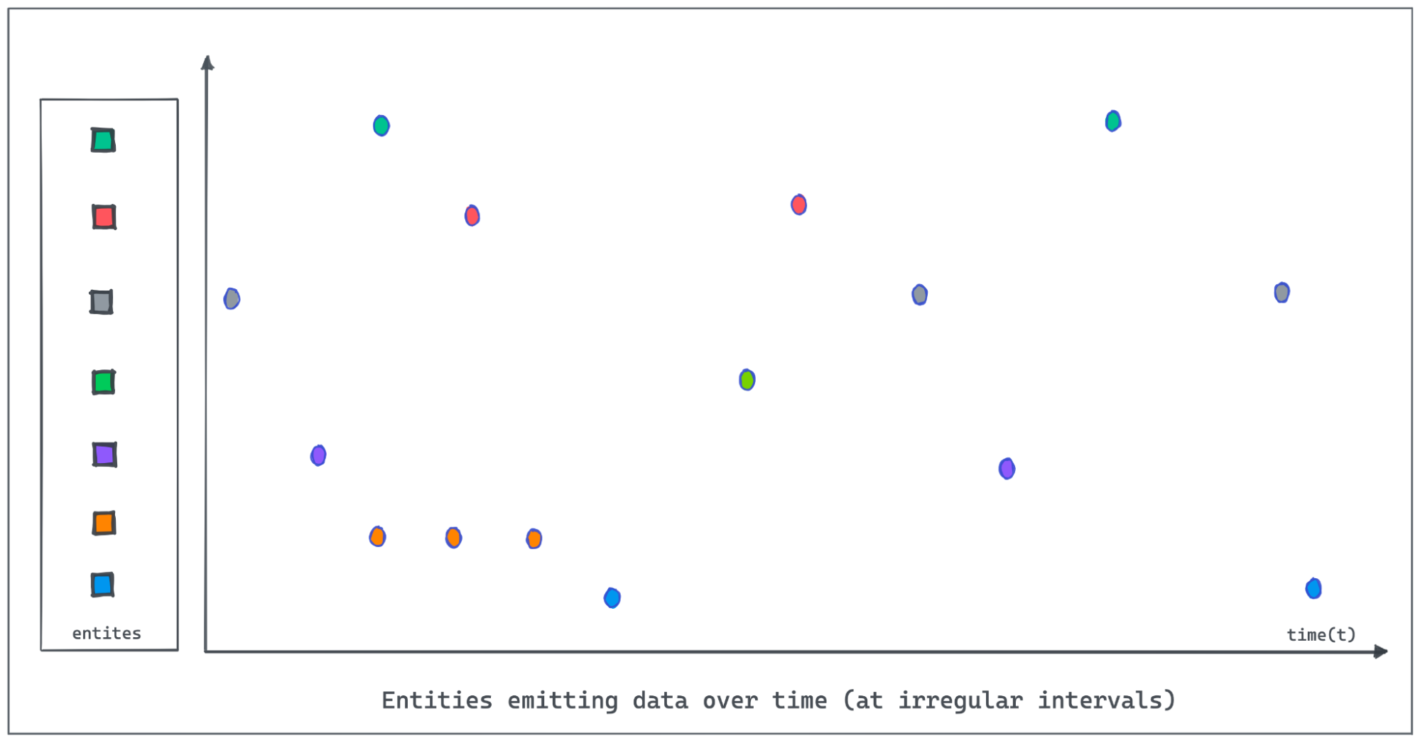
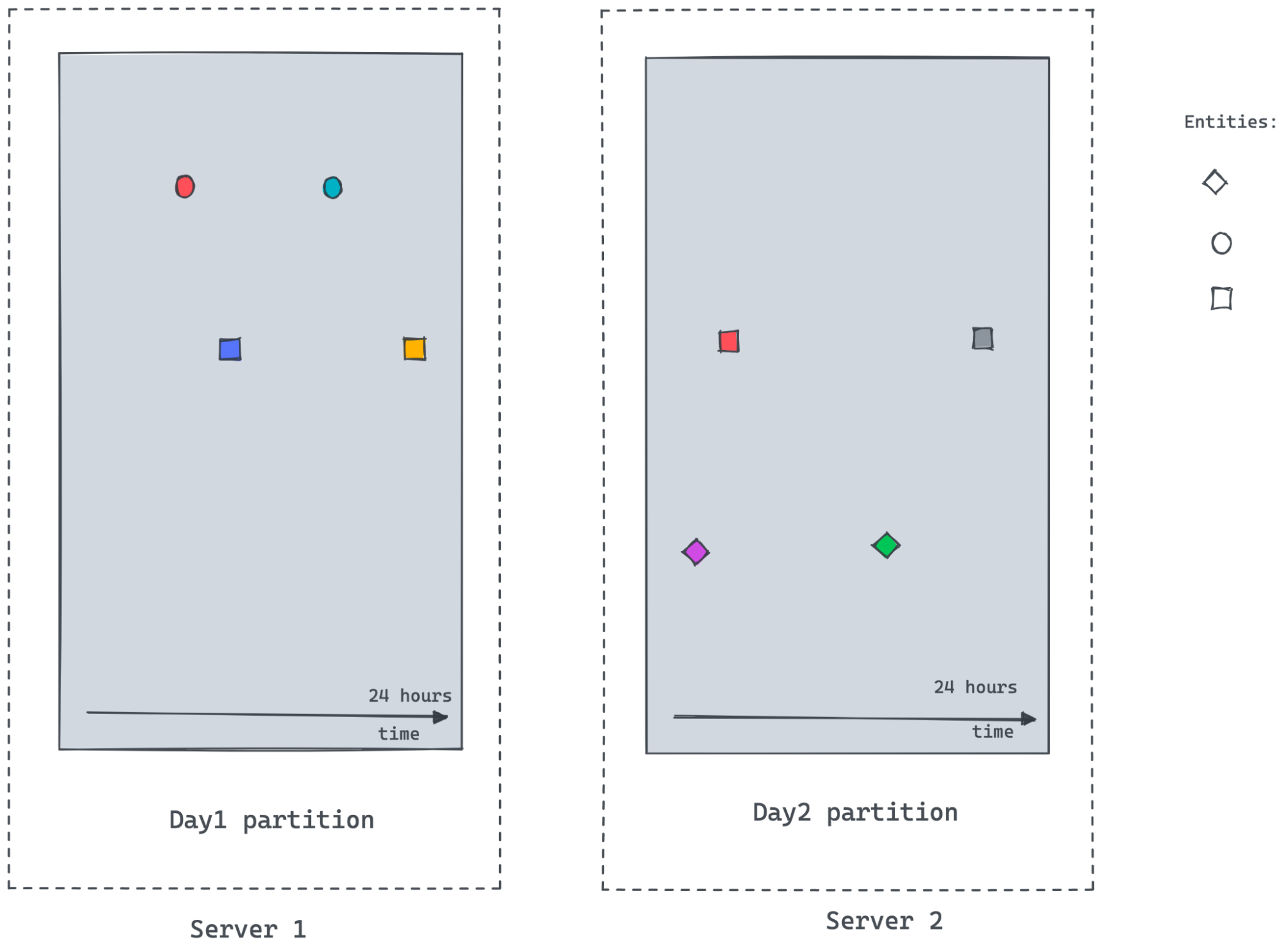
Let us use an IOT dataset tracking the occupancy status of the individual
parking slots in a parking garage using automated sensors in this post. The
granularity of recorded data points might be sparse or the events could be
missing due to network and other device issues in the IOT environment. The
following figure demonstrates entities emitting values at irregular intervals
as the value changes. Polling and recording values of all entities regularly at
a lower granularity would consume [...]
-
+
It is important for Pinot to provide the on-the-fly interpolation (filling the
missing data) functionality to better handle time-series data.
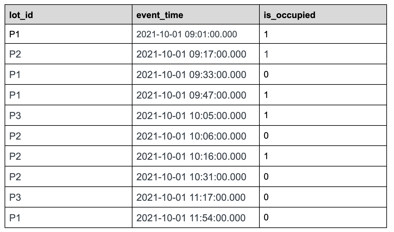
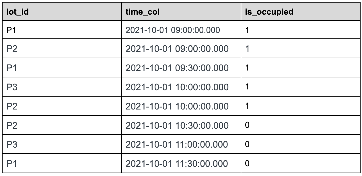
@@ -32,7 +32,7 @@ Let us use the following sample data set tracking the status
of parking lots in
### Sample Dataset:
-
+
parking_data table
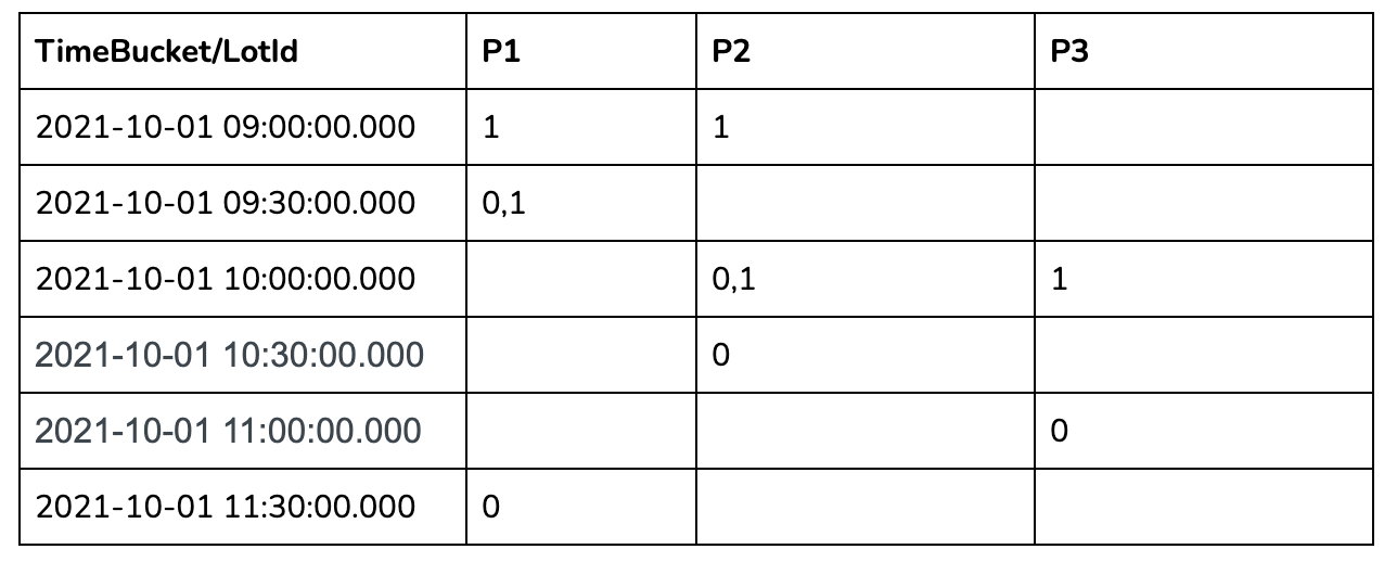
@@ -40,7 +40,7 @@ Use case: We want to find out the total number of parking
lots that are occupie
Let us take 30 minutes time bucket as an example:
-
+
In the 30 mins aggregation results table above, we can see a lot of missing
data as many lots didn't have anything recorded in those 30-minute windows. To
calculate the number of occupied parking lots per time bucket, we need to
gap-fill the missing data for each of these 30-minute windows.
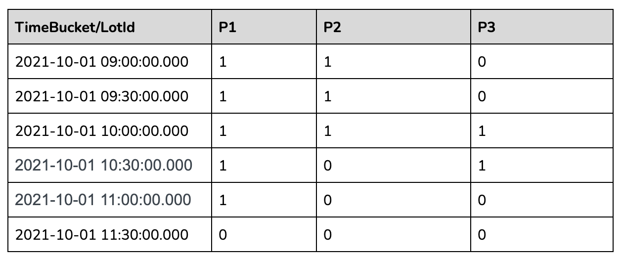
@@ -100,15 +100,15 @@ The following concepts were added to interpolate and
handle time-series data.
The innermost sql will convert the raw event table to the following table.
-
+
The second most nested sql will gap fill the returned data as below:
-
+
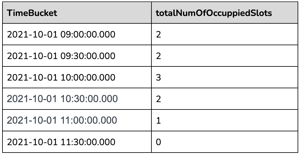
The outermost query will aggregate the gapfilled data as follows:
-
+
### Other Supported Query Scenarios:
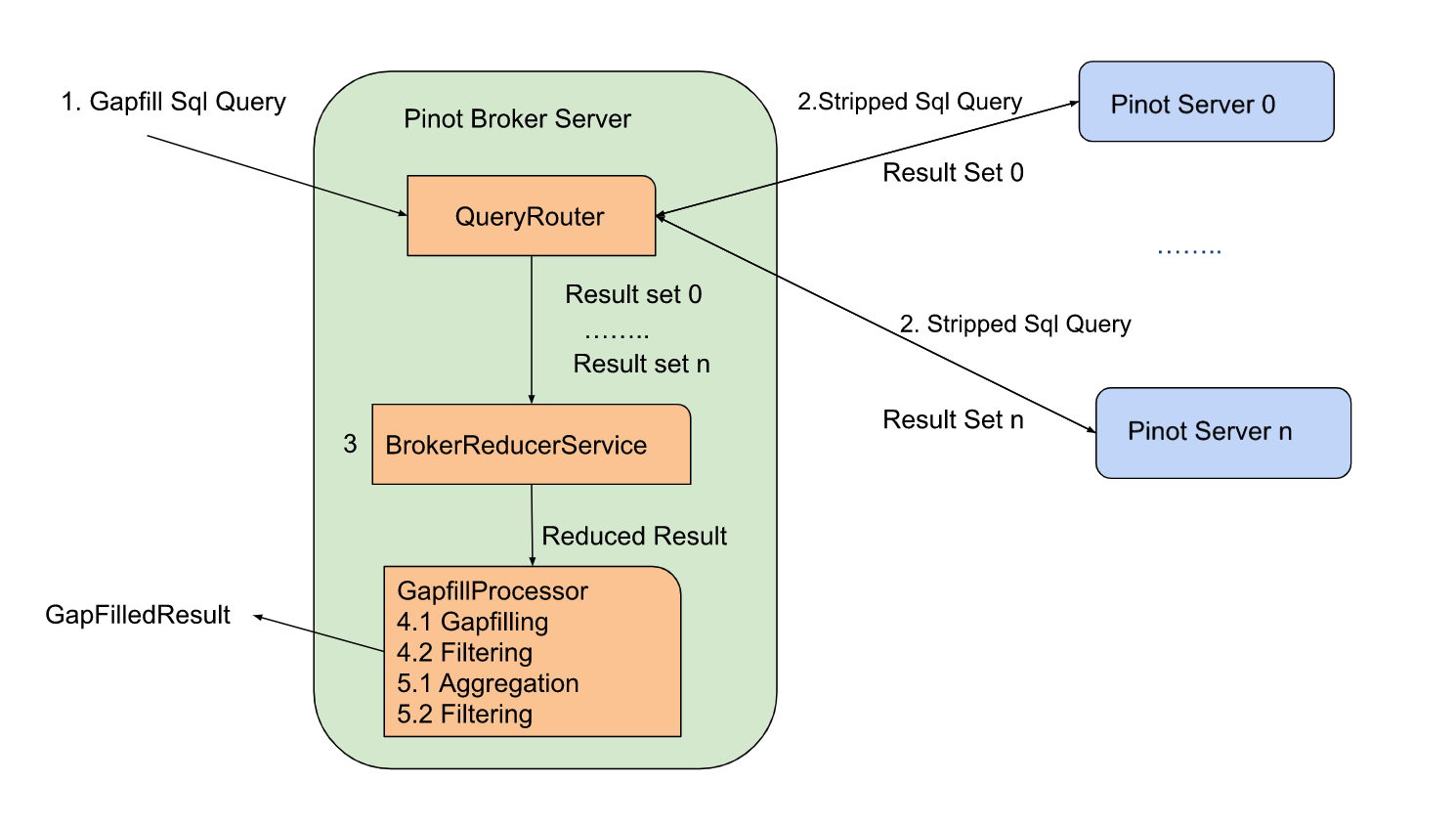
@@ -139,7 +139,7 @@ There are two gapfill-specific steps:
1. When Pinot Broker Server receives the gapfill SQL query, it will strip out
gapfill related information and send out the stripped SQL query to the pinot
server
2. GapfillProcessor will process the result from BrokerReducerService. The
gapfill logic will be applied to the reduced result.
-
+
Here is the stripped version of the sql query sent to servers for the query
shared above:
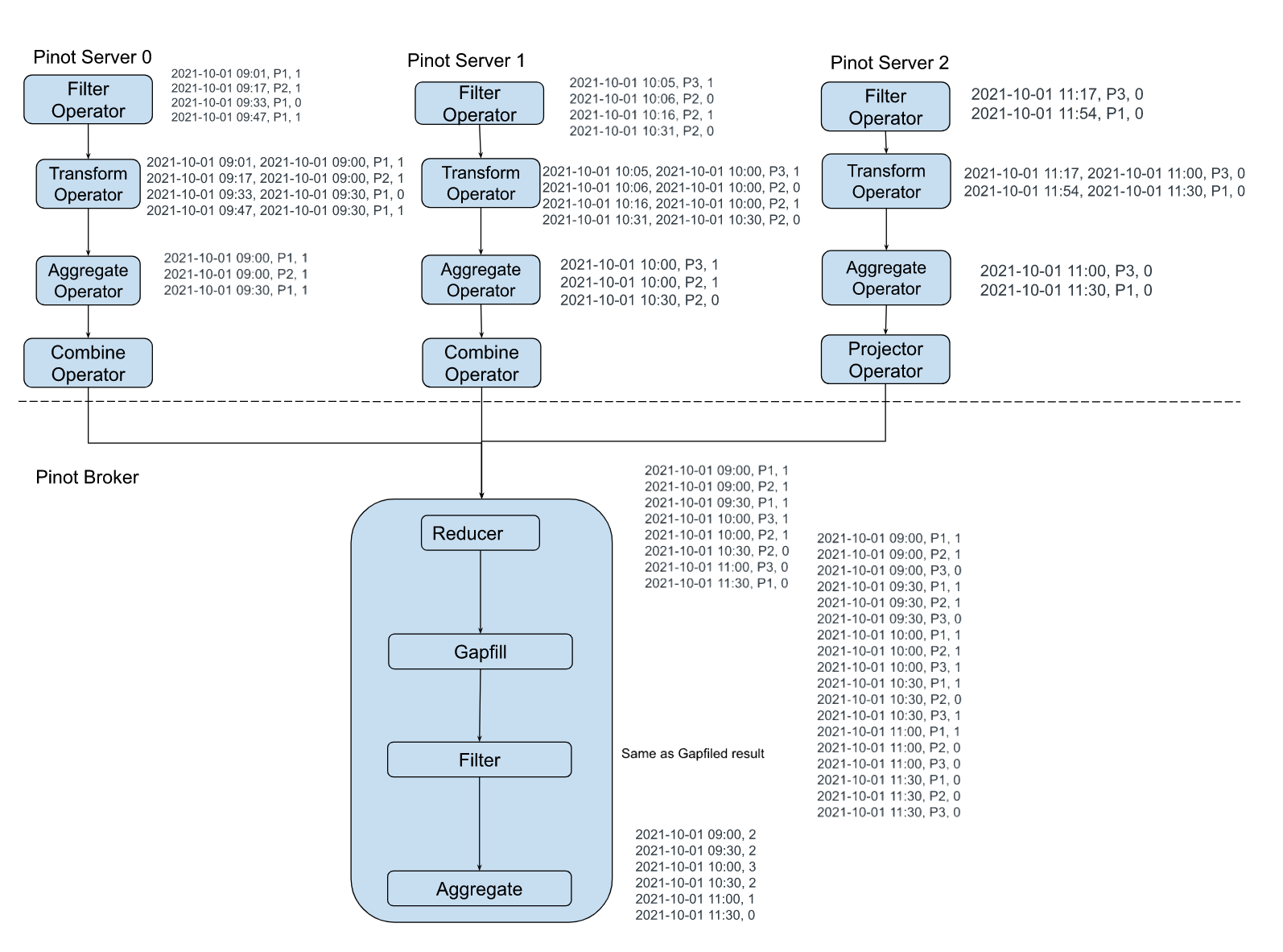
@@ -158,7 +158,7 @@ SELECT DATETIMECONVERT(event_time,'1:MILLISECONDS:EPOCH',
The sample execution plan for this query is as shown in the figure below:
-
+
### Time and Space complexity:
@@ -166,7 +166,7 @@ Let us say there are M entities, R rows returned from
servers, and N time bucket
### Challenges
-
+
As the time-series datasets are enormous and partitioned, it's hard to get
answers to the following questions:
diff --git a/data/blog/2022-11-08-Apache Pinot-How-do-I-see-my-indexes.mdx
b/data/blog/2022-11-08-Apache Pinot-How-do-I-see-my-indexes.mdx
index 48444ecc..68c529ad 100644
--- a/data/blog/2022-11-08-Apache Pinot-How-do-I-see-my-indexes.mdx
+++ b/data/blog/2022-11-08-Apache Pinot-How-do-I-see-my-indexes.mdx
@@ -36,11 +36,11 @@ docker run \
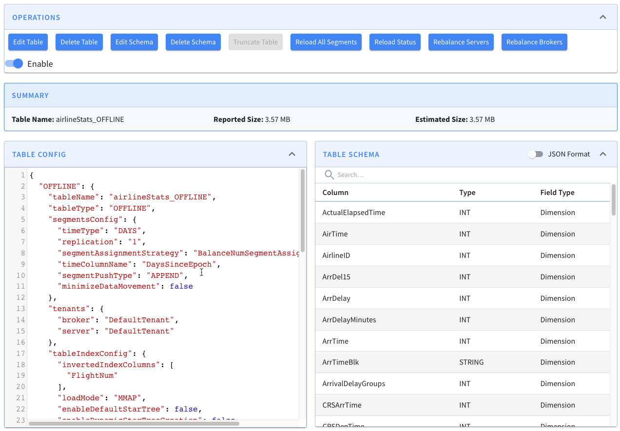
Once that’s up and running, navigate to
[http://localhost:9000/#/](http://localhost:9000/#/) and click on Tables. Under
the tables section click on airlineStats_OFFLINE. You should see a page that
looks like this:
-
+
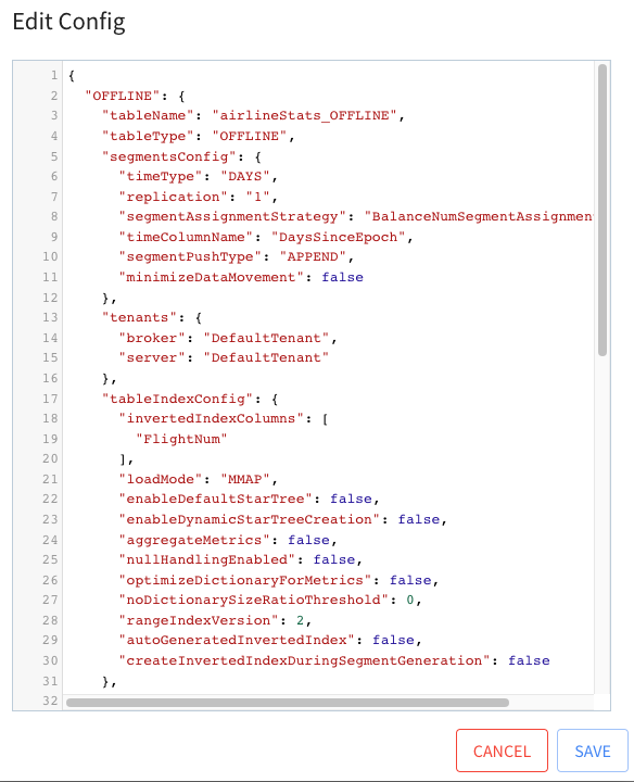
Click on Edit Table. This will show a window with the config for this table.
-
+
## Indexing Config
@@ -98,7 +98,7 @@ Now, close the table config modal, and under the segments
section, open airlineS
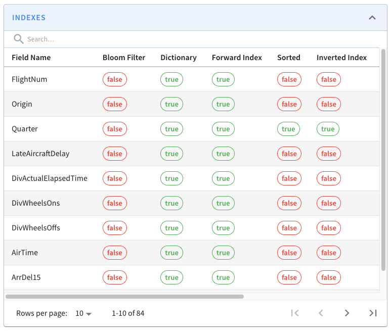
If you look at one of those segments, you’ll see the following grid that lists
columns/field names against the indexes defined on those fields.
-
+
All the fields on display are persisting their values using the
dictionary/forward [index
format](https://docs.pinot.apache.org/basics/indexing/forward-index) ). Still,
we can also see that the Quarter column is sorted and has an inverted index,
neither of which we explicitly defined.
@@ -112,11 +112,11 @@ I’ve written a couple of blog posts explaining how sorted
indexes work on offl
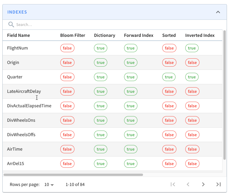
Next, let’s see what happens if we add an explicit index. We’re going to add
an inverted index to the FlightNum column. Go to Edit Table config again and
update tableIndexConfig to have the following value:
-
+
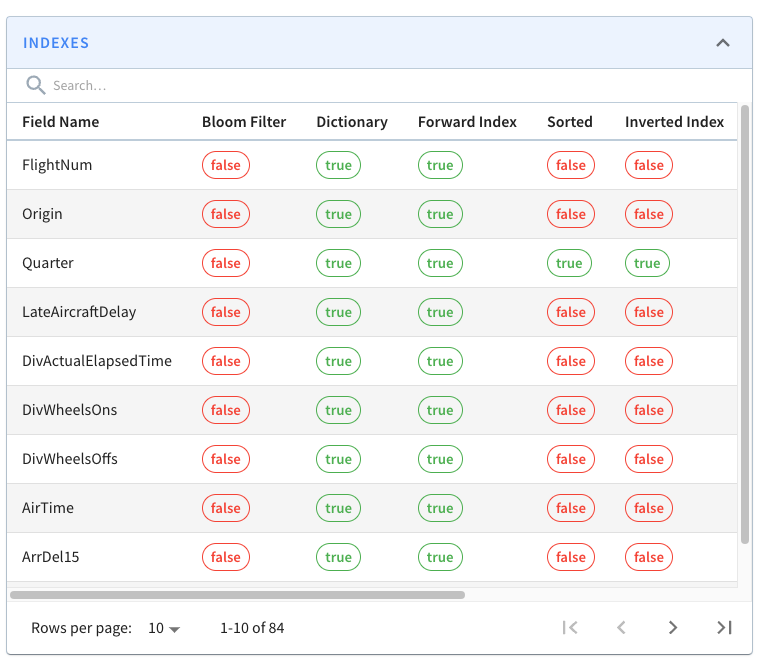
If you go back to the page for segment airlineStats_OFFLINE_16073_16073_0,
notice that it does not have an inverted index for this field.
-
+
This is because indexes are applied on a per segment basis. If we want the
inverted index on the FlightNum column in this segment, we can click _Reload
Segment_ on this page, or we can go back to the table page and click _Reload
All Segments_.
diff --git a/data/blog/2022-11-17-Apache Pinot-Inserts-from-SQL.mdx
b/data/blog/2022-11-17-Apache Pinot-Inserts-from-SQL.mdx
index 8abcce6f..5036f288 100644
--- a/data/blog/2022-11-17-Apache Pinot-Inserts-from-SQL.mdx
+++ b/data/blog/2022-11-17-Apache Pinot-Inserts-from-SQL.mdx
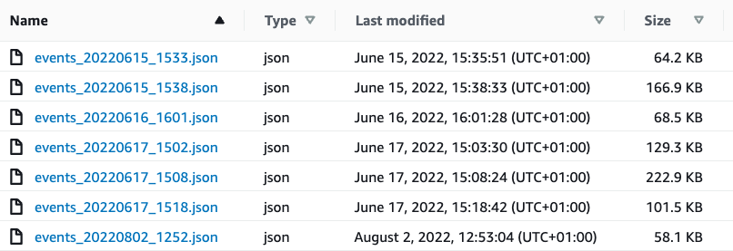
@@ -20,11 +20,11 @@ In the [Batch Import JSON from Amazon S3 into Apache Pinot
| StarTree Recipes](h
The contents of that bucket are shown in the screenshot below:
-
+
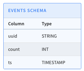
Let’s quickly recap the steps that we had to do to import those files into
Pinot. We have a table called events, which has the following schema:
-
+
We first created a job specification file, which contains a description of our
import job. The job file is shown below:
@@ -74,7 +74,7 @@ And don’t worry, those credentials have already been deleted;
I find it easier
Once we’ve run this command, if we go to the Pinot UI at
[http://localhost:9000](http://localhost:9000/) and click through to the events
table from the Query Console menu, we’ll see that the records have been
imported, as shown in the screenshot below:
-
+
This approach works, and we may still prefer to use it when we need
fine-grained control over the ingestion parameters, but it is a bit heavyweight
for your everyday data import!
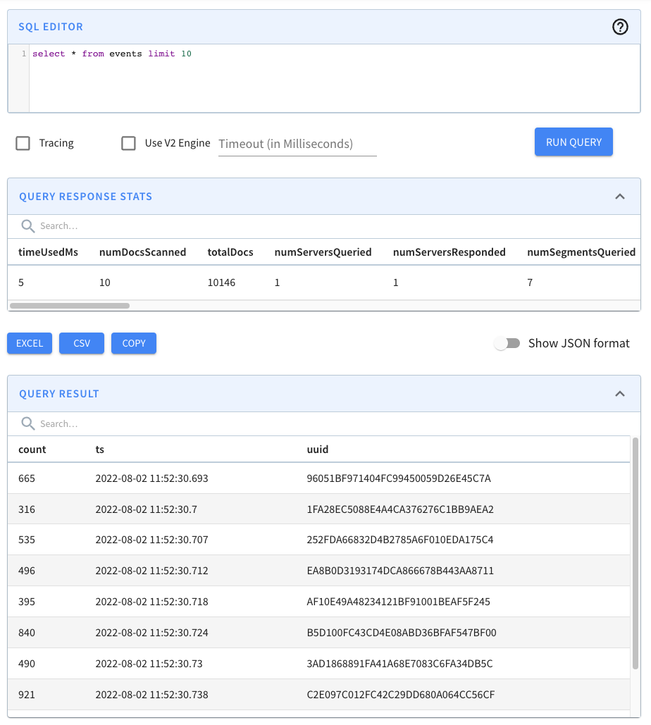
@@ -111,11 +111,11 @@ OPTION(
If we run this query, we’ll see the following output:
-
+
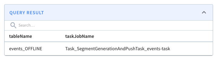
We can check on the state of the ingestion job via the Swagger REST API. If we
navigate to
[http://localhost:9000/help#/Task/getTaskState](http://localhost:9000/help#/Task/getTaskState),
paste Task_SegmentGenerationAndPushTask_events-task as our task name, and then
click Execute, we’ll see the following:
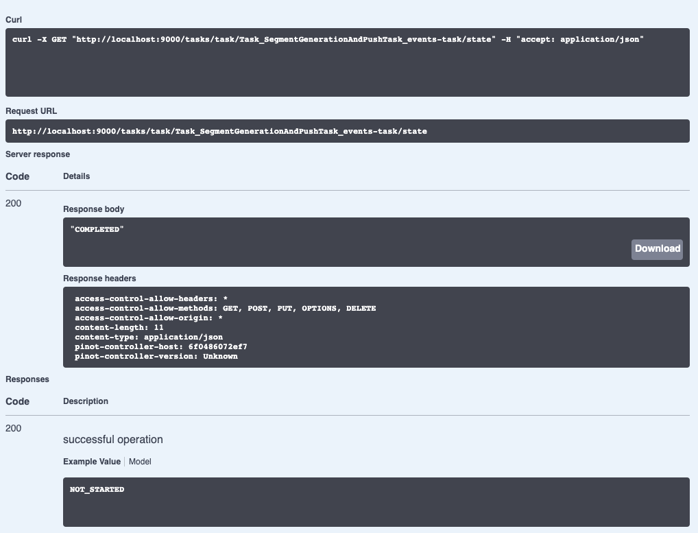
-
+
If we see the state COMPLETED, this means the data has been ingested, which we
can check by going back to the Query console and clicking on the events table.
diff --git a/data/blog/2022-11-22-Apache-Pinot-Timestamp-Indexes.mdx
b/data/blog/2022-11-22-Apache-Pinot-Timestamp-Indexes.mdx
index 3df02852..ceeb6d31 100644
--- a/data/blog/2022-11-22-Apache-Pinot-Timestamp-Indexes.mdx
+++ b/data/blog/2022-11-22-Apache-Pinot-Timestamp-Indexes.mdx
@@ -20,7 +20,7 @@ Instead, users write queries that use the datetrunc function
to filter at a coar
The [timestamp
index](https://docs.pinot.apache.org/basics/indexing/timestamp-index) solves
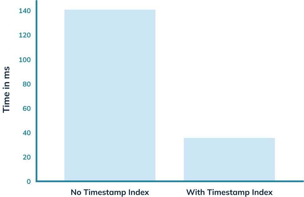
that problem! In this blog post, we’ll use it to get an almost 5x query speed
improvement on a relatively small dataset of only 7m rows.
-
+
## Spinning up Pinot
@@ -86,7 +86,7 @@ We should see the following output:
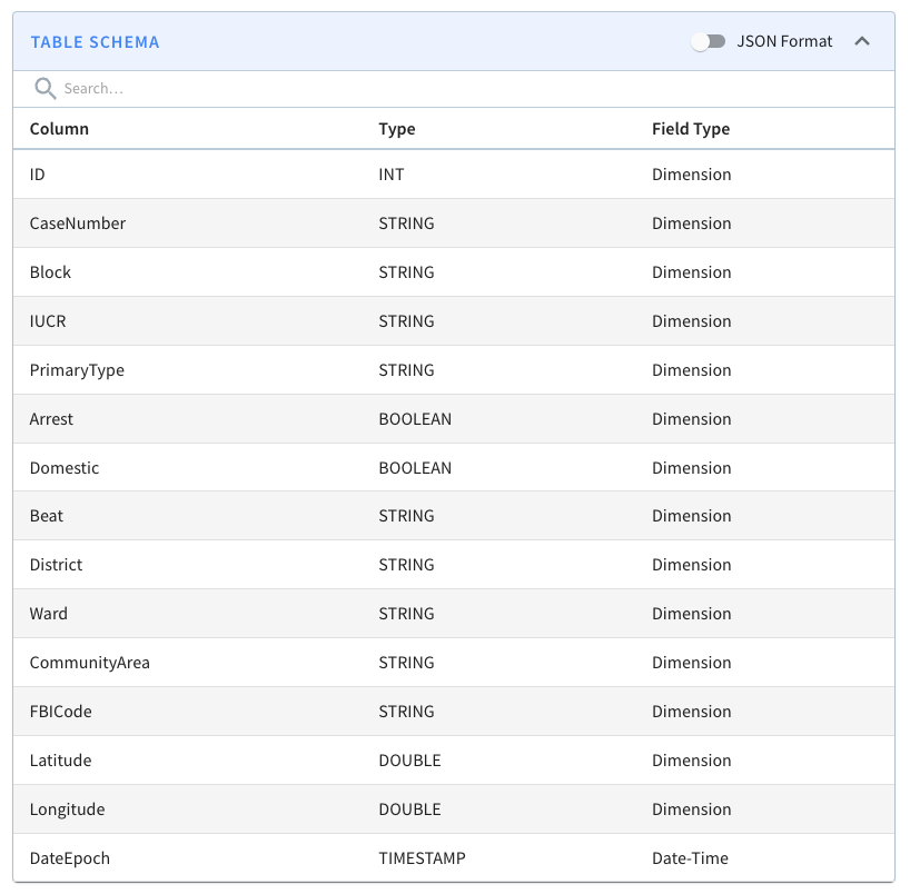
A screenshot of the schema is shown below:
-
+
We won’t go through the table config and schema files in this blog post
because we did that in the last post, but you can find them in the
[config](https://github.com/startreedata/pinot-recipes/tree/main/recipes/analyzing-chicago-crimes/config)
directory on GitHub.
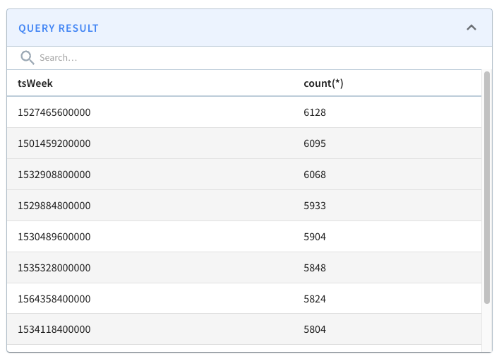
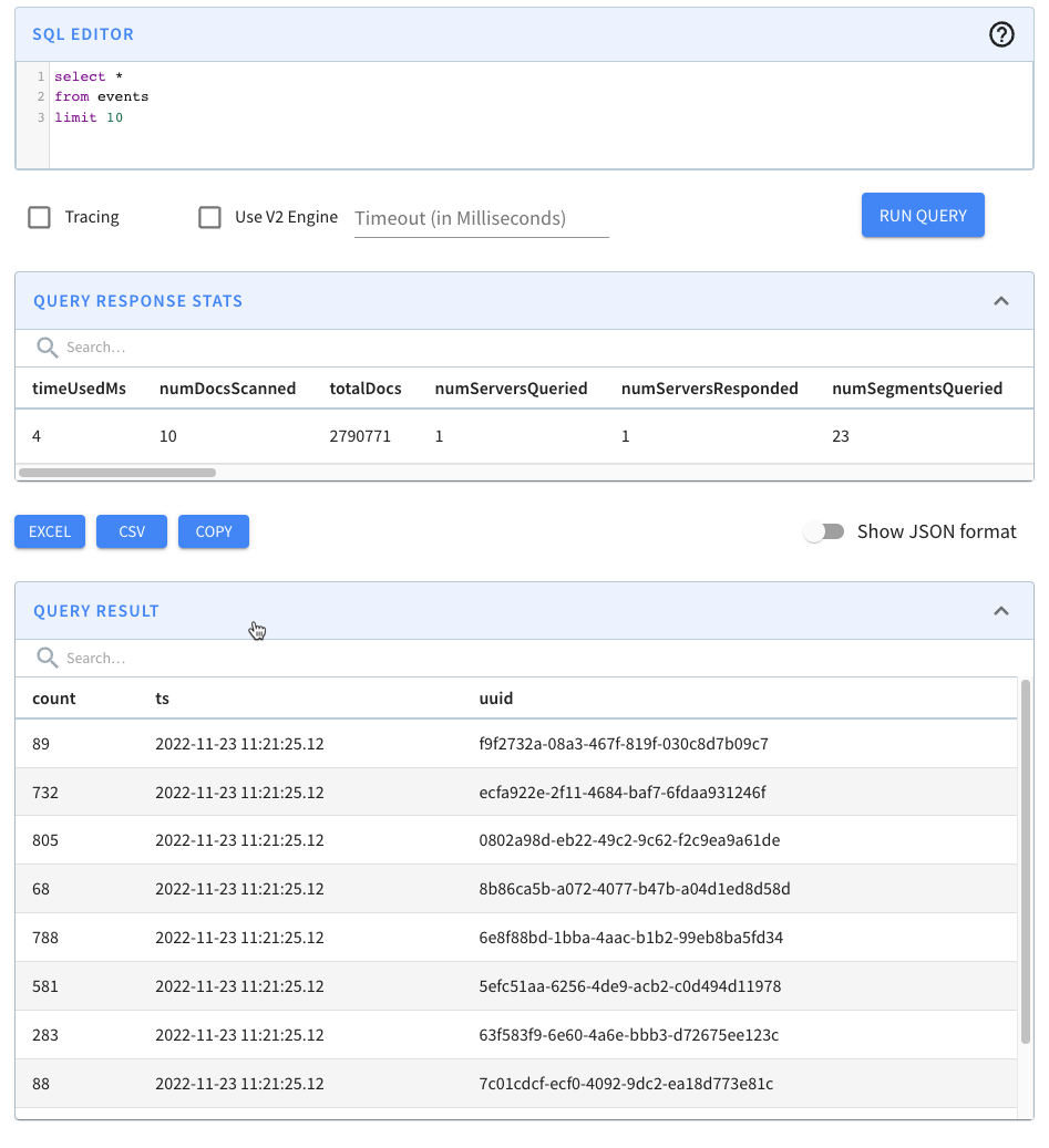
@@ -119,11 +119,11 @@ limit 10
If we run that query, we’ll see the following results:
-
+
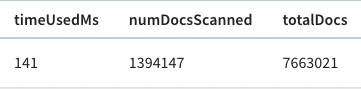
And, if we look above the query result, there’s metadata about the query,
including the time that it took to run.
-
+
The query took 141 ms to execute, so that’s our baseline.
@@ -222,7 +222,7 @@ In our case, that means we’ll have these extra columns:
$DateEpoch$DAY, $DateE
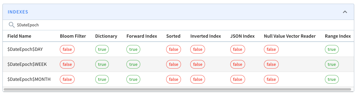
We can check if the extra columns and indexes have been added by navigating to
the
[segment_page](http://localhost:9000/#/tenants/table/crimes_indexed_OFFLINE/crimes_OFFLINE_0)
and typing $Date$Epoch in the search box. You should see the following:
-
+
These columns will be assigned the following values:
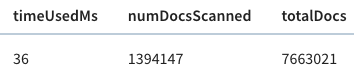
@@ -276,7 +276,7 @@ limit 10
Let’s now run our initial query against the _crimes_indexed_ table. We’ll get
exactly the same results as before, but let’s take a look at the query stats:
-
+
This time the query takes 36 milliseconds rather than 140 milliseconds. That’s
an almost 5x improvement, thanks to the timestamp index.
diff --git a/data/blog/2022-11-28-Apache-Pinot-Pausing-Real-Time-Ingestion.mdx
b/data/blog/2022-11-28-Apache-Pinot-Pausing-Real-Time-Ingestion.mdx
index 40e4bce0..5b4976b9 100644
--- a/data/blog/2022-11-28-Apache-Pinot-Pausing-Real-Time-Ingestion.mdx
+++ b/data/blog/2022-11-28-Apache-Pinot-Pausing-Real-Time-Ingestion.mdx
@@ -26,7 +26,7 @@ Once a segment reaches the [segment
threshold,](https://dev.startree.ai/docs/pin
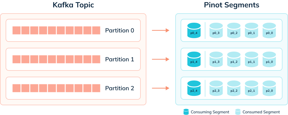
The diagram below shows what things might look like when we’re ingesting data
from a Kafka topic that has 3 partitions:
-
+
A table has one consuming segment per partition but would have many completed
segments.
@@ -298,7 +298,7 @@ This time we will see some consuming segments:
Navigate to [http://localhost:9000/#/query](http://localhost:9000/#/query) and
click on the events table. You should see the following:
-
+
We have records! We can also run our data generator again, and more events
will be ingested.
diff --git
a/data/blog/2023-01-29-Apache-Pinot-Deduplication-on-Real-Time-Tables.mdx
b/data/blog/2023-01-29-Apache-Pinot-Deduplication-on-Real-Time-Tables.mdx
index f3cfa33f..25d7b5ce 100644
--- a/data/blog/2023-01-29-Apache-Pinot-Deduplication-on-Real-Time-Tables.mdx
+++ b/data/blog/2023-01-29-Apache-Pinot-Deduplication-on-Real-Time-Tables.mdx
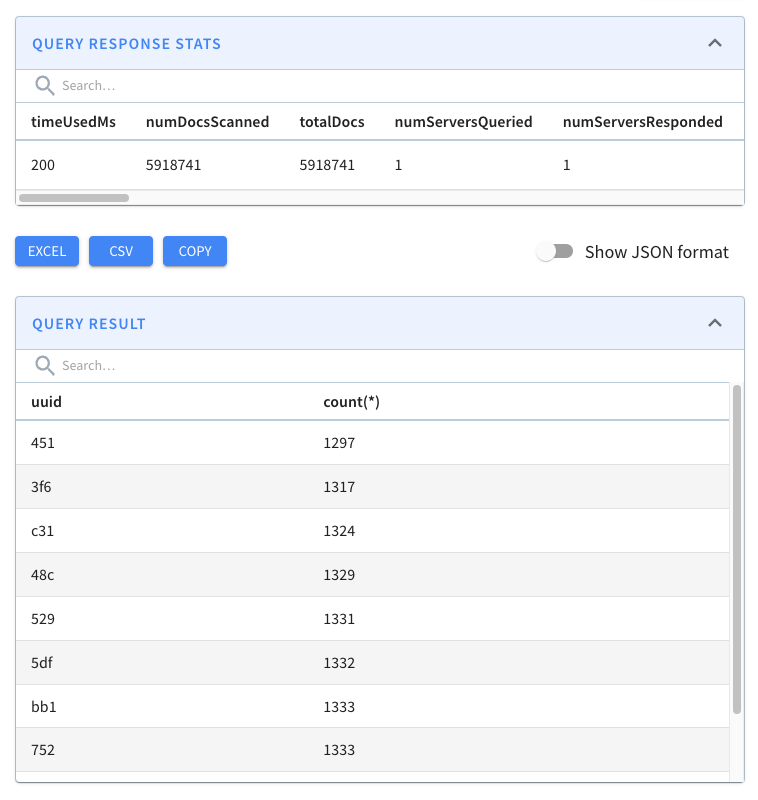
@@ -245,7 +245,7 @@ limit 10
The results of this query are shown below:
-
+
We can see loads of duplicates!
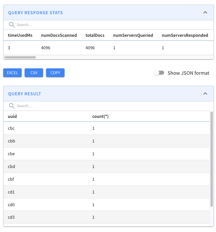
@@ -331,7 +331,7 @@ The changes to notice here are:
limit 10
```
-
+
We have every combination of hex values (16^3=4096) and no duplicates! Pinot’s
de-duplication feature has done its job.
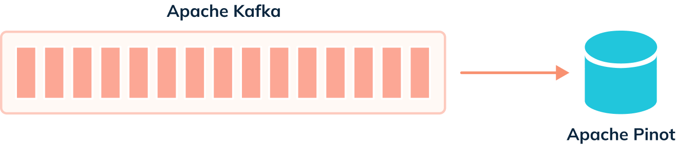
@@ -339,11 +339,11 @@ We have every combination of hex values (16^3=4096) and
no duplicates! Pinot’s
When we’re not using the deduplication feature, events are ingested from our
streaming platform into Pinot, as shown in the diagram below:
-
+
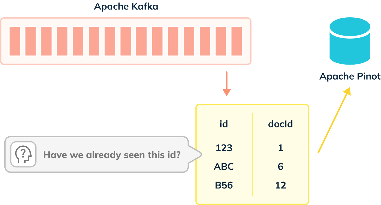
When de-dup is enabled, we have to check whether records can be ingested, as
shown in the diagram below:
-
+
De-dup works out whether a primary key has already been ingested by using an
in memory map of (primary key -> corresponding segment reference).
diff --git
a/data/blog/2023-02-21-Apache-Pinot-0-12-Configurable-Time-Boundary.mdx
b/data/blog/2023-02-21-Apache-Pinot-0-12-Configurable-Time-Boundary.mdx
index 887ece48..5ec3749a 100644
--- a/data/blog/2023-02-21-Apache-Pinot-0-12-Configurable-Time-Boundary.mdx
+++ b/data/blog/2023-02-21-Apache-Pinot-0-12-Configurable-Time-Boundary.mdx
@@ -32,7 +32,7 @@ The ingestion frequency can either be 1 hour or 1 day, so one
of these values wi
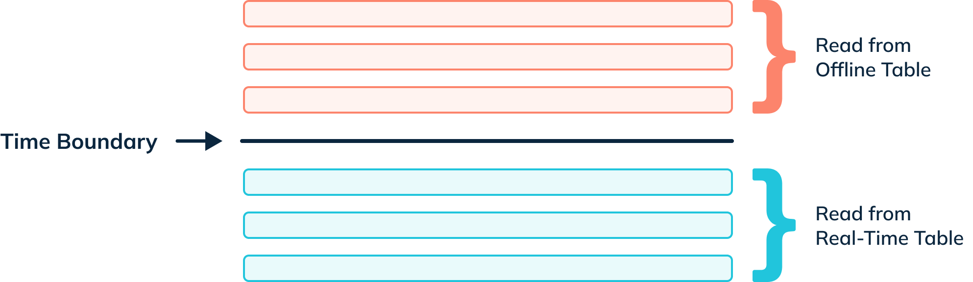
When a query for a hybrid table is received by a Pinot Broker, the broker
sends a time boundary annotated version of the query to the offline and
real-time tables. Any records from or before the time boundary are read from
the offline table; anything greater than the boundary comes from the real-time
table.
-
+
For example, if we executed the following query:
diff --git a/data/blog/2023-03-30-Apache-Pinot-0-12-Consumer-Record-Lag.mdx
b/data/blog/2023-03-30-Apache-Pinot-0-12-Consumer-Record-Lag.mdx
index e0145211..16e57da9 100644
--- a/data/blog/2023-03-30-Apache-Pinot-0-12-Consumer-Record-Lag.mdx
+++ b/data/blog/2023-03-30-Apache-Pinot-0-12-Consumer-Record-Lag.mdx
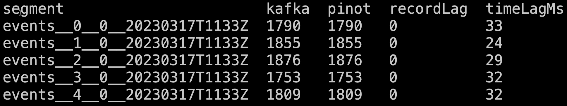
@@ -211,7 +211,7 @@ Let’s call the function:
We’ll see the following output:
-
+
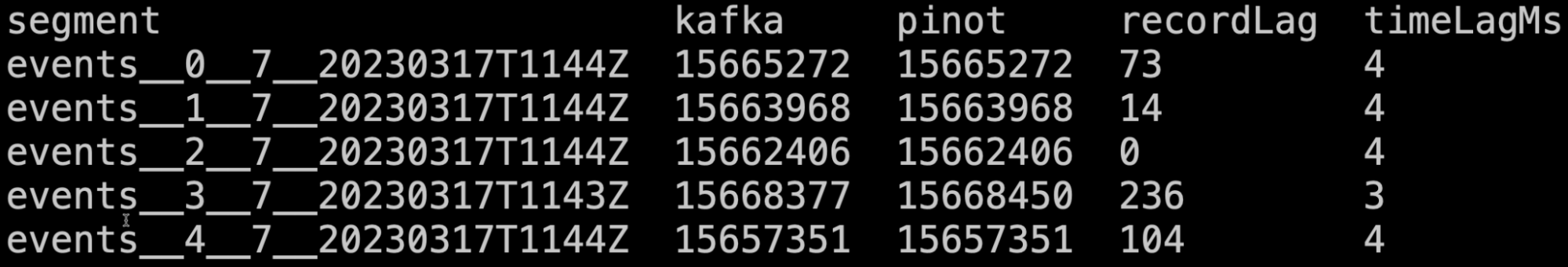
Now let’s put it in a script and call the watch command so that it will be
refreshed every couple of seconds:
@@ -253,7 +253,7 @@ kcat -P -b localhost:9092 -t events -Kø
And now if we look at the watch output:
-
+
We get some transitory lag, but it generally goes away by the next time the
command is run.
diff --git a/data/blog/2023-05-11-Geospatial-Indexing-in-Apache-Pinot.mdx
b/data/blog/2023-05-11-Geospatial-Indexing-in-Apache-Pinot.mdx
index 77149451..e96246f8 100644
--- a/data/blog/2023-05-11-Geospatial-Indexing-in-Apache-Pinot.mdx
+++ b/data/blog/2023-05-11-Geospatial-Indexing-in-Apache-Pinot.mdx
@@ -28,7 +28,7 @@ We can index points using [H3](https://h3geo.org/), an open
source library that
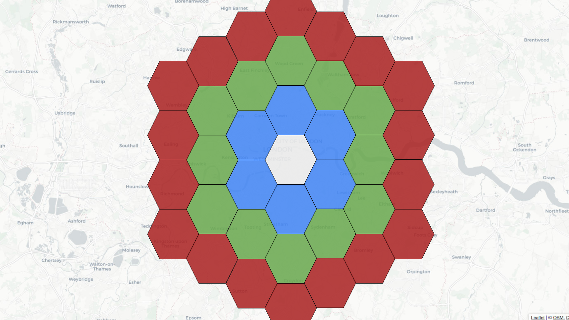
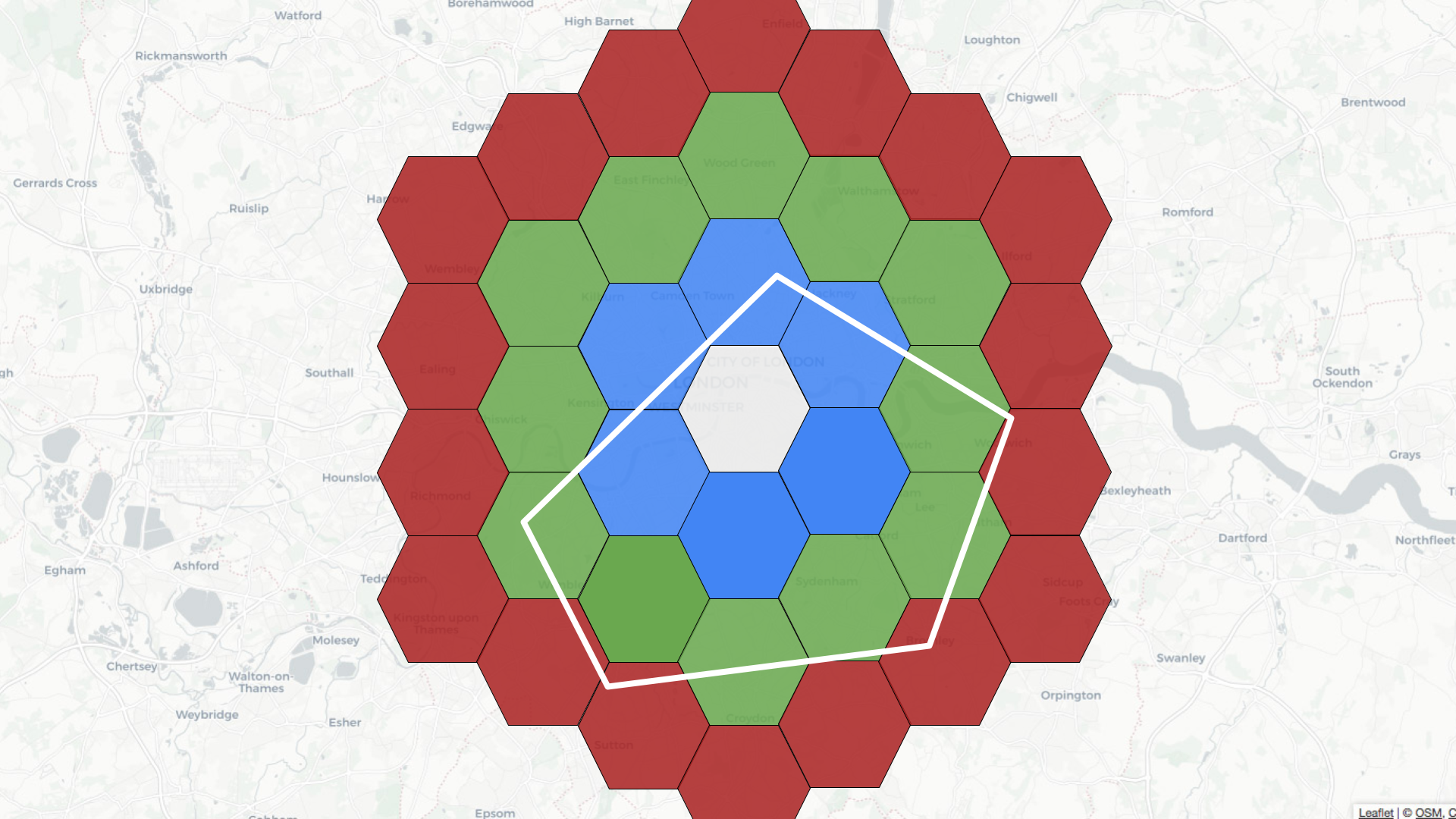
For example, if the central hexagon covers the Westminster area of central
London, neighbors at distance 1 are colored blue, those at distance 2 are in
green, and those at distance 3 are in red.
-
+
Let’s learn how to use geospatial indexing with help from a dataset that
captures the latest location of trains moving around the UK. We’re streaming
this data into a `trains` topic in Apache Kafka®. Here’s one message from this
stream:
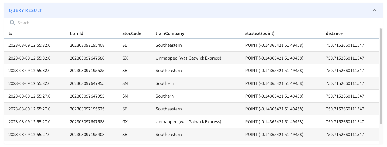
@@ -146,13 +146,13 @@ limit 10
These results from running the query would follow:
-
+
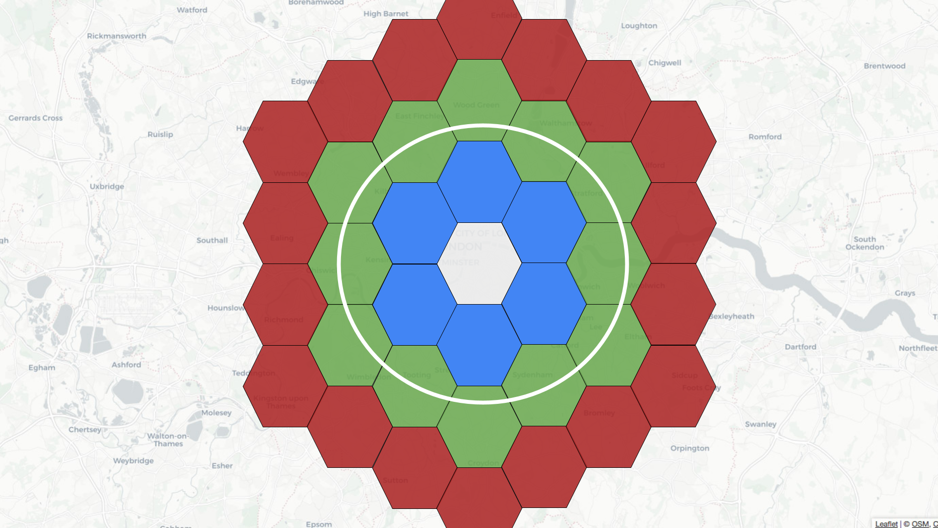
Let’s now go into a bit more detail about what happens when we run the query.
The 10 km radius covers the area inside the white circle on the diagram below:
-
+
Pinot’s query planner will first translate the distance of 10 km into a number
of rings, in this case, two. It will then find all the hexagons located two
rings away from the white one. Some of these hexagons will fit completely
inside the white circle, and some will overlap with the circle.
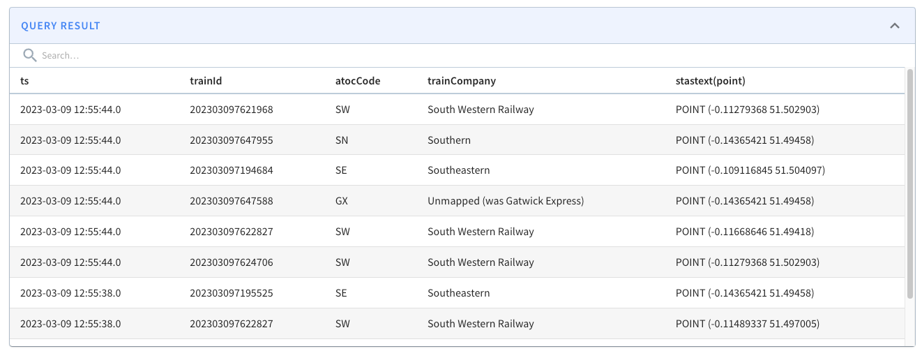
@@ -182,17 +182,17 @@ limit 10
The results from running the query are shown below:
-
+
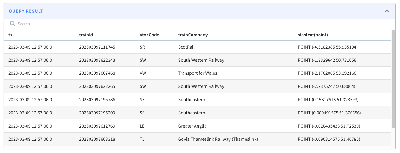
If we change the query to show trains outside of a central London polygon,
we’d see the following results:
-
+
So what’s actually happening when we run this query?
The polygon covers the area inside the white shape as shown below:
-
+
Pinot’s query planner will first find all the coordinates on the exterior of
the polygon. It will then find the hexagons that fit within that geofence.
Those hexagons get added to the potential cells list.
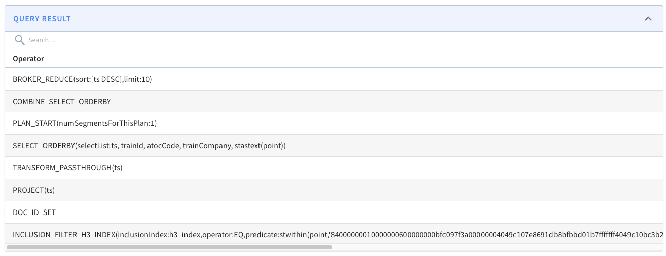
@@ -231,7 +231,7 @@ If our query uses `STDistance`, we should expect to see the
`FILTER\_H3\_I
See this example query plan:
-
+
The [StarTree Developer Hub](https://dev.startree.ai/) contains a [geospatial
indexing
guide](https://dev.startree.ai/docs/pinot/recipes/geospatial-indexing#how-do-i-check-that-the-geospatial-index-is-being-used)
that goes through this in more detail.
diff --git
a/data/blog/2023-05-16-star-tree-indexes-in-apache-pinot-part-1-understanding-the-impact-on-query-performance.mdx
b/data/blog/2023-05-16-star-tree-indexes-in-apache-pinot-part-1-understanding-the-impact-on-query-performance.mdx
index b5235937..81f2ed81 100644
---
a/data/blog/2023-05-16-star-tree-indexes-in-apache-pinot-part-1-understanding-the-impact-on-query-performance.mdx
+++
b/data/blog/2023-05-16-star-tree-indexes-in-apache-pinot-part-1-understanding-the-impact-on-query-performance.mdx
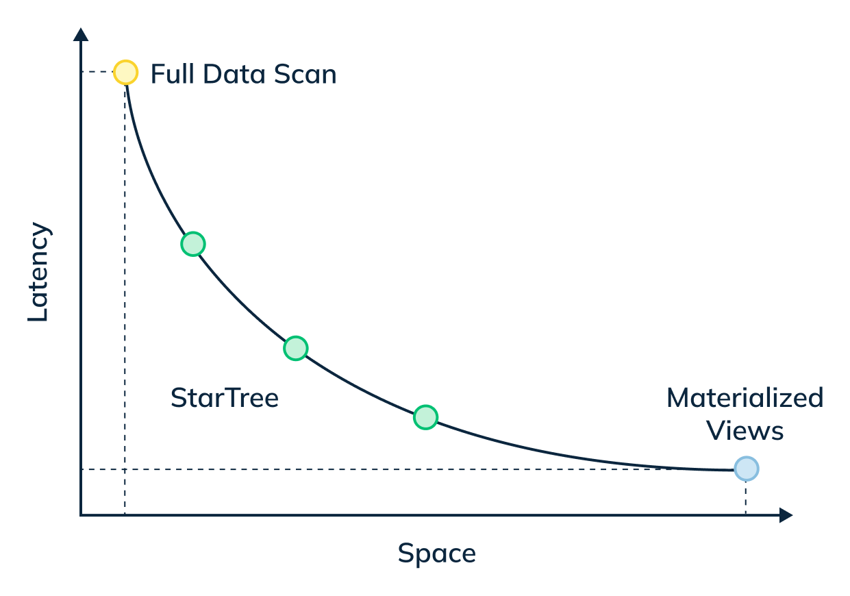
@@ -16,31 +16,31 @@ _Star-Tree Index: Pinot’s Intelligent Materialized View:_
_The star-tree index provides an intelligent way to build materialized views
within Pinot. Traditional MVs work by fully materializing the computation for
each source record that matches the specified predicates. Although useful, this
can result in non-trivial storage overhead. On the other hand, the star-tree
index allows us to partially materialize the computations and provide the
ability to tune the space-time tradeoff by providing a configurable threshold
between pre-aggregation and [...]
-
+
In this three-part blog series, we will compare and contrast query performance
of a star-tree index with an inverted index, something that most of the OLAP
databases end up using for such queries.
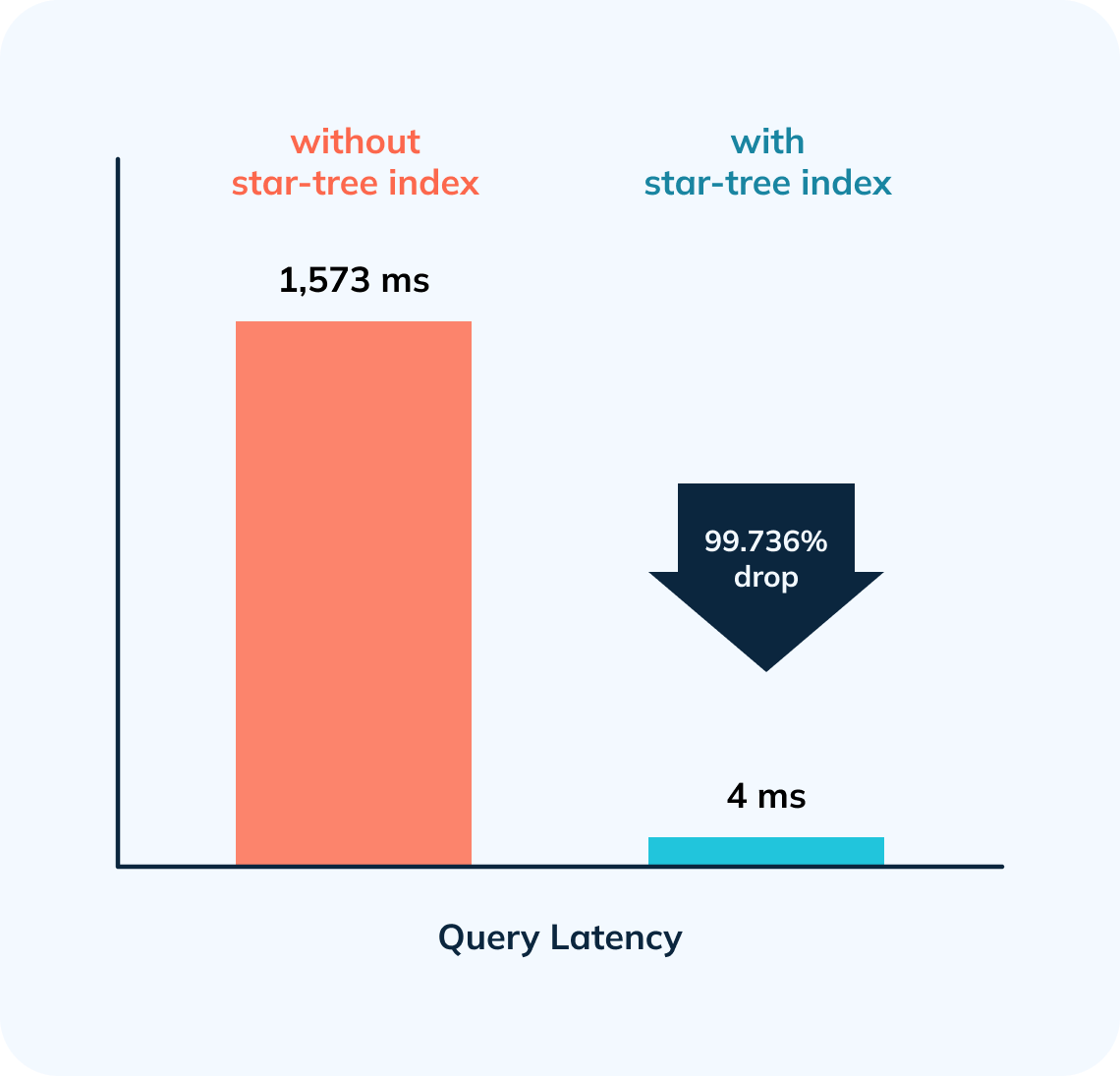
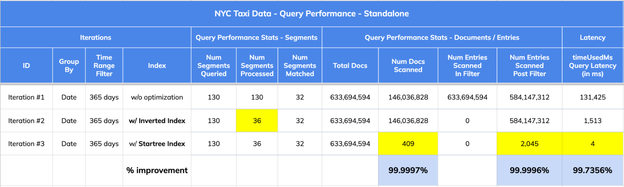
In this first part, we will showcase how a star-tree index brought down
standalone query latency on a sizable dataset of ~633M records from 1,513ms to
4ms! — nearly 380x faster.
-
+
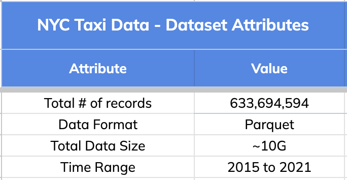
## 1\. The Dataset:
We used New York City Taxi Data for this comparison. Original source:
[here](https://www.kaggle.com/c/nyc-taxi-trip-duration). Below are the high
level details about this dataset.
-
+
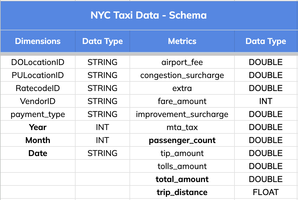
### Schema:
The dataset has 8 dimension fields and 11 metric columns as listed below.
-
+
## 2\. Query Pattern
The query pattern involved slicing and dicing the data (GROUPING) BY various
dimensions (Date, Month and Year), aggregating different metrics (total trips,
distance and passengers count) and FILTERING BY a time range that could go as
wide as 1 year.
-
+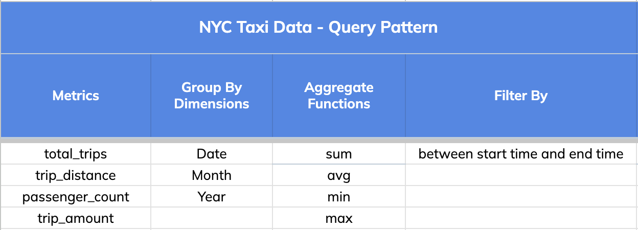
Note: A key thing to note is that a single star-tree index covers a wide range
of OLAP queries that comprise the dimensions, metrics and aggregate functions
specified in it.
@@ -92,7 +92,7 @@ We will use one such variant query for this illustration:
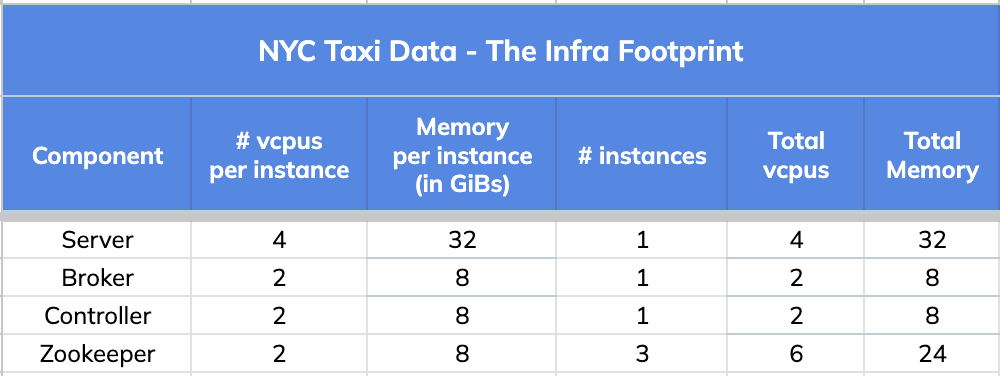
We used a very small infrastructure footprint for this comparison test.
-
+
## 4\. Query Results and Stats
@@ -148,7 +148,7 @@ limit 1000
option(useStarTree=false, timeoutMs=20000)
```
-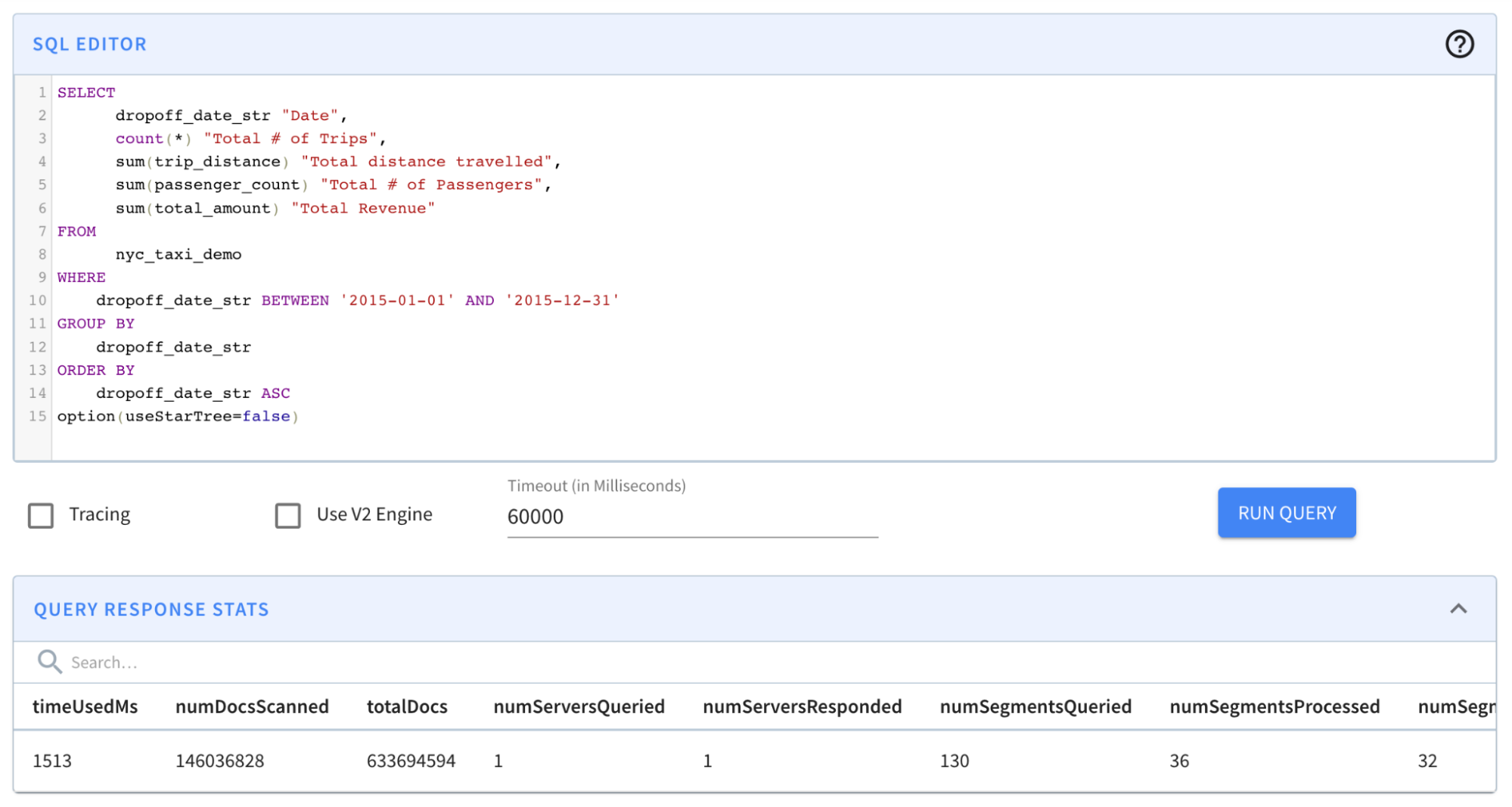
+
Result: The query completed in 1,513 milliseconds. (~1.5s); from ~131s to
~1.5s was a BIG improvement. However, results still took more than a second —
which is a relatively long time for an OLAP database, especially if it is faced
with multiple concurrent queries.
@@ -176,7 +176,7 @@ limit 1000
option(useStarTree=true)
```
-
+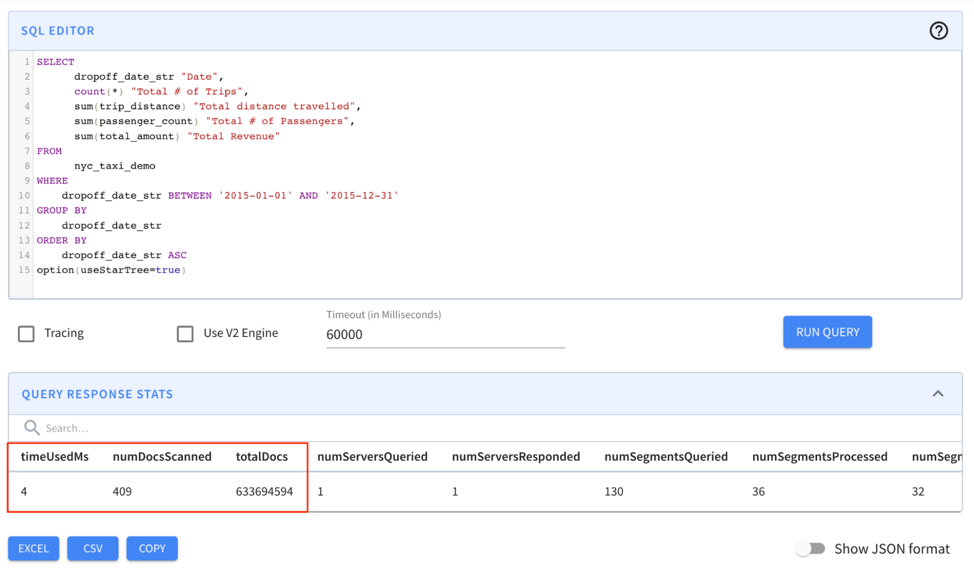
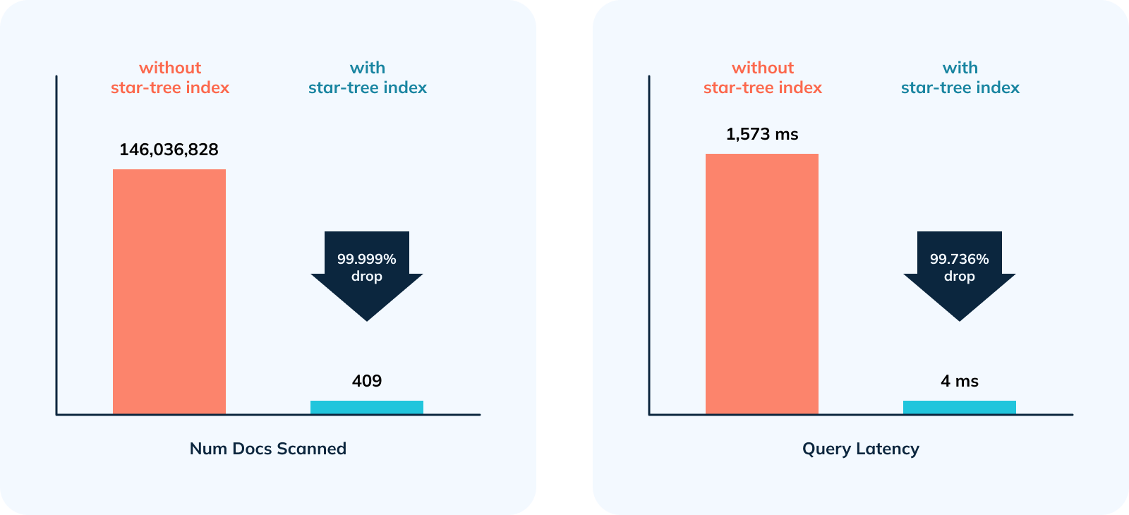
Result: The query completed in 4 milliseconds! Notice in particular that the
numDocsScanned came down from ~146M to 409!
@@ -184,7 +184,7 @@ Result: The query completed in 4 milliseconds! Notice in
particular that the num
Let’s take a closer look at the [query response
stats](https://docs.pinot.apache.org/users/api/querying-pinot-using-standard-sql/response-format)
across all three iterations to understand the “how” part of this magic of
indexing in Apache Pinot.
-
+
1. The dataset has 633,694,594 records (documents) spread across 130 segments.
2. Query Stats:
@@ -195,7 +195,7 @@ Let’s take a closer look at the [query response
stats](https://docs.pinot.apac
## 5\. Impact Summary:
-
+
1. 356,968x improvement (or 99.999% drop) in num docs scanned from ~146M to
409.
2. 378.5x improvement (~99.736% drop) in query latency from 1,513 ms to 4 ms.
diff --git
a/data/blog/2023-05-18-apache-pinot-tutorial-for-getting-started-a-step-by-step-guide.mdx
b/data/blog/2023-05-18-apache-pinot-tutorial-for-getting-started-a-step-by-step-guide.mdx
index c3ac4088..331dcbac 100644
---
a/data/blog/2023-05-18-apache-pinot-tutorial-for-getting-started-a-step-by-step-guide.mdx
+++
b/data/blog/2023-05-18-apache-pinot-tutorial-for-getting-started-a-step-by-step-guide.mdx
@@ -53,7 +53,7 @@ _Docker is a set of platform as a service (PaaS) products
that use OS-level virt
Now, let’s download the Docker image. On a Windows machine, start a new
PowerShell command window. Note that this is not the same as a Windows
PowerShell command window, as shown below.
-
+
Use the following command to get (pull) the image we are looking for:
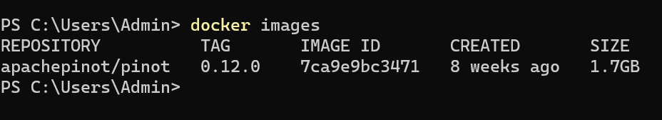
@@ -79,7 +79,7 @@ docker images
It should show you the image like so:
-
+
### Step 3:
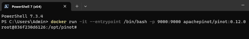
@@ -89,7 +89,7 @@ Let’s run a container using the Docker image that we
downloaded:
docker run -it --entrypoint /bin/bash -p 9000:9000
apachepinot.docker.scarf.sh/apachepinot/pinot:0.12.0
```
-
+
The docker run command runs the image. The \-p 9000:00 option maps the docker
container port 9000 to the local machine port 9000. This allows us to access
the Pinot UI, which defaults to port 9000 to be accessible from the localhost.
We are using the –entrypoint to override the default entrypoint and replace it
with Bash. We want to override the default behavior so that we can start each
component one at a time. The next parameter
apachepinot.docker.scarf.sh/apachepinot/pinot:0.12.0 is t [...]
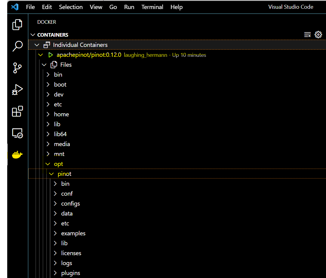
@@ -97,7 +97,7 @@ After running the command, we’ll find ourselves in the Docker
container instan
If you’re using VS Code, with the Docker extension installed, you can click on
the Docker extension and see our container and its content:
-
+
Click on the Docker icon in the left menu, and
apachepinot.docker.scarf.sh/apachepinot/pinot:0.12.0. This should take a few
seconds to connect to the running container. Now, you can navigate to the files
and see what we have under the opt folder.
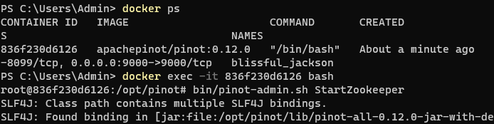
@@ -105,7 +105,7 @@ Click on the Docker icon in the left menu, and
apachepinot.docker.scarf.sh/apach
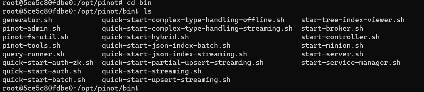
Let’s run the components that are essential to running a Pinot cluster. Change
directory to the bin folder and list the contents like so:
-
+
In order to start the Pinot cluster, we will need to run the following
essential components:
@@ -134,7 +134,7 @@ The controller controls the cluster health and coordinates
with ZooKeeper for co
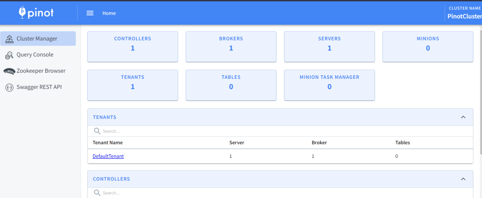
At this time, we should have a running Pinot cluster. We can verify via the
Pinot Data Explorer by browsing to localhost:9000. You should see something
like this:
-
+
What just happened?
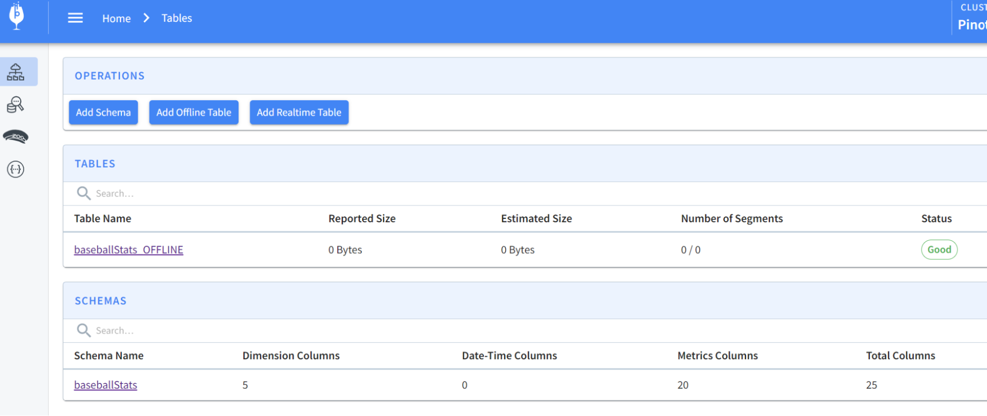
@@ -206,7 +206,7 @@ To create a schema and table for the baseball stats file,
run the following comm
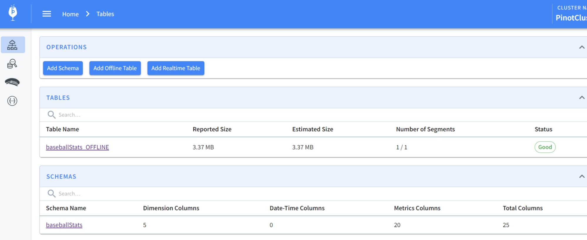
You should now see the schema and table created:
-
+
Next, we’ll want to load some data into the table that we created. We have
some sample data in the folder rawdata that we can use to load. We will need a
YAML file to perform the actual ingestion job and can use the following command
to import data:
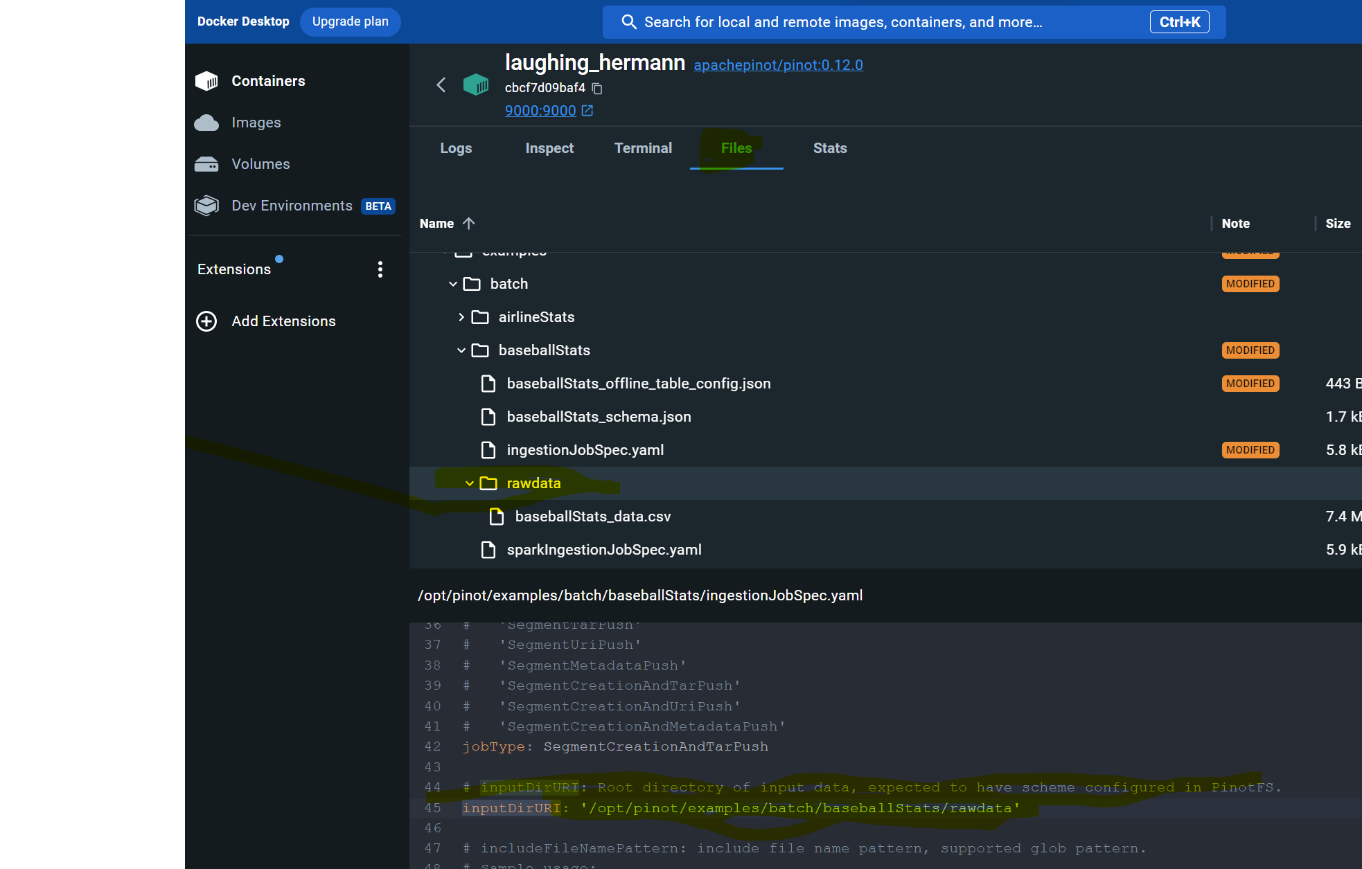
@@ -217,11 +217,11 @@ Next, we’ll want to load some data into the table that we
created. We have som
If you run into trouble on this step like I did, edit the ingestJobSpec.yaml
file using Docker Desktop to change the inputDirURI from relative to absolute
path. Then rerun the above command.
-
+
You should now be able to see the table has been populated like so:
-
+
Now, let’s run some queries. From localhost:9000, select the Query Console in
the left-hand menu. Then type in some of these queries:
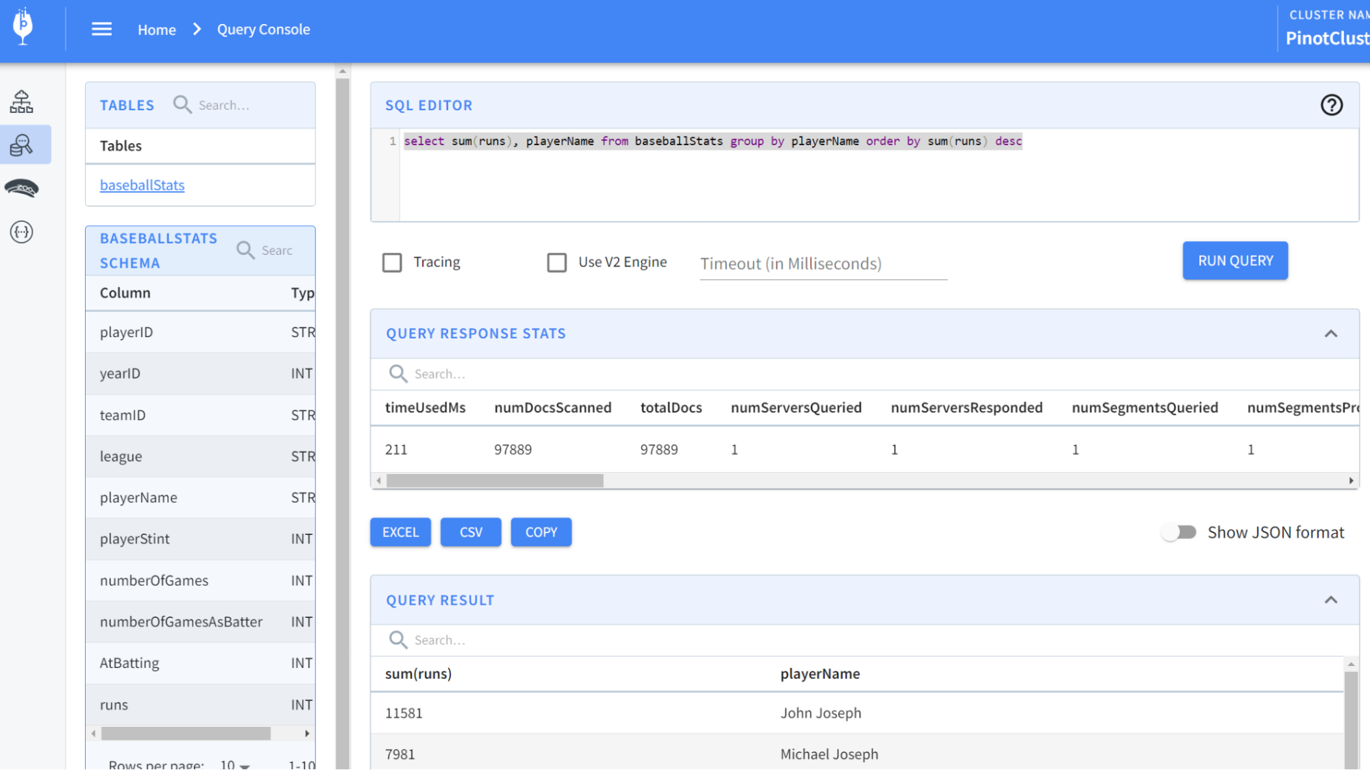
@@ -232,7 +232,7 @@ select sum(runs), playerName from baseballStats group by
playerName order by sum
You should see results like so:
-
+
And there you have it!
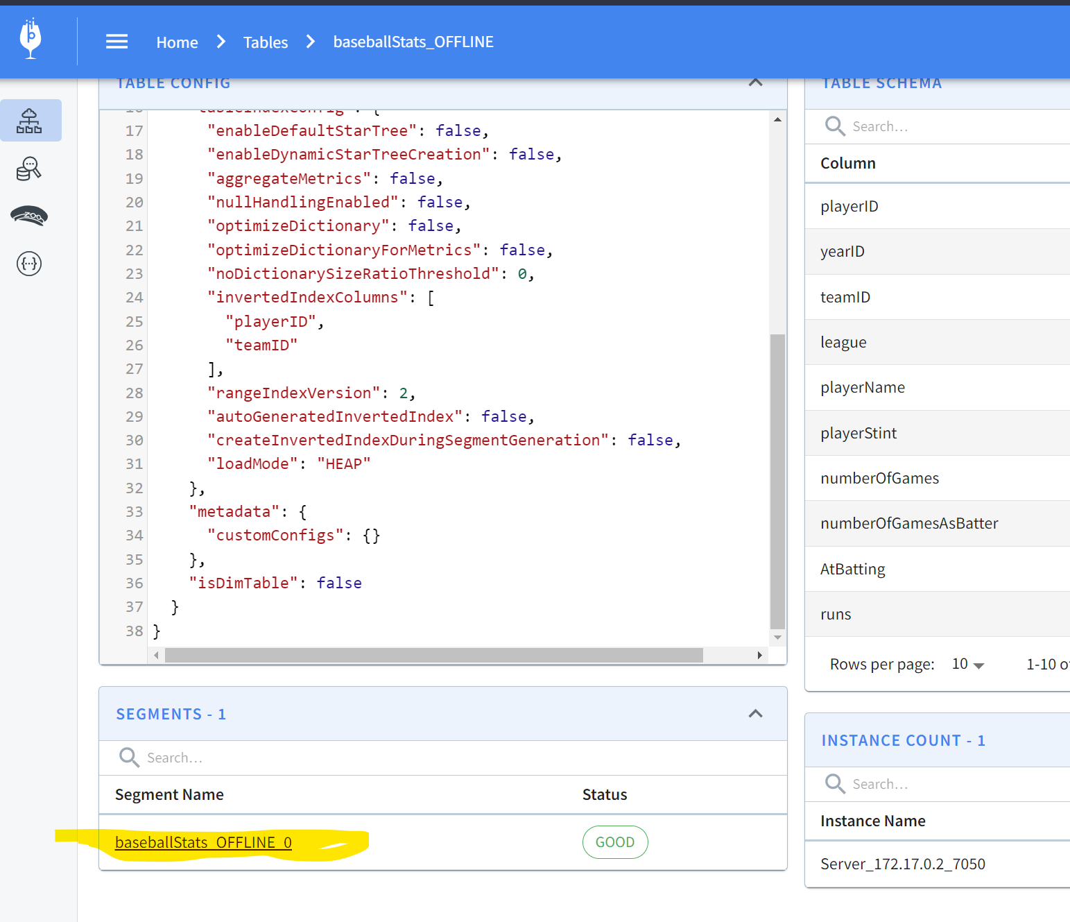
@@ -240,11 +240,11 @@ And there you have it!
If you’re curious to go a step further and see what the segments look like and
what the actual data on disk looks like, keep reading! In the Tables section of
localhost:9000, you can scroll down to find a segment:
-
+
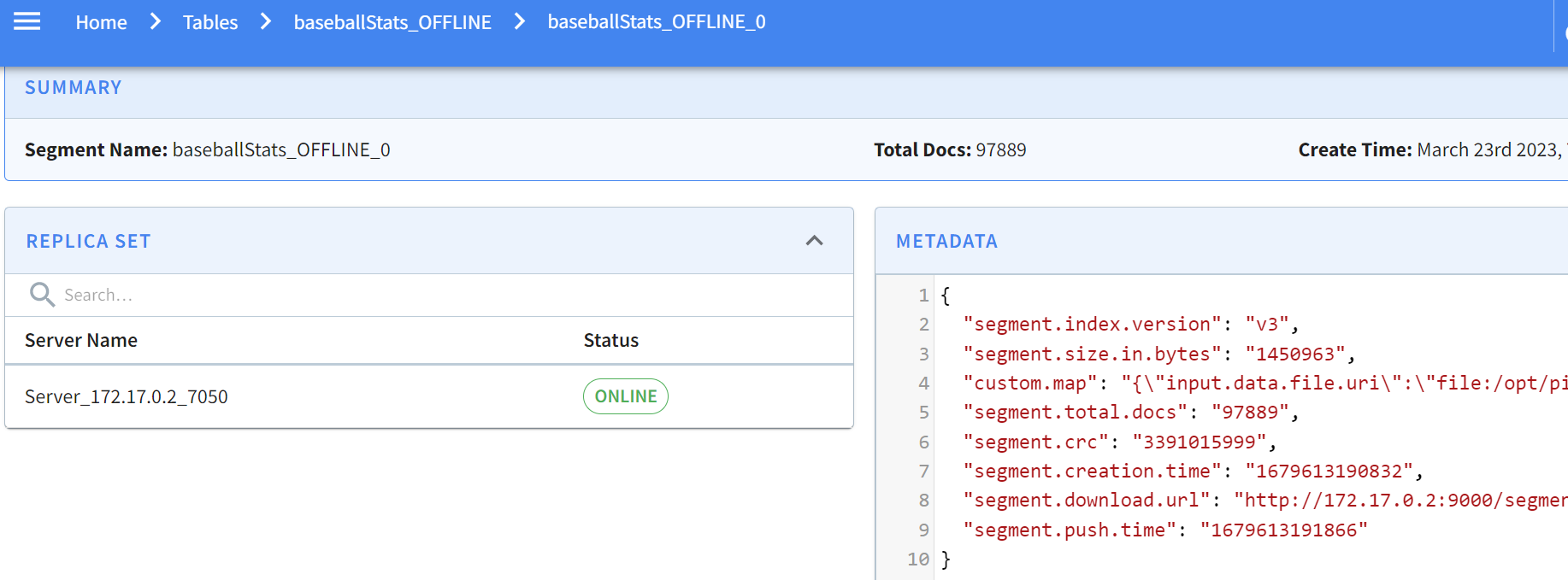
Clicking on this gives the specifics of the segment:
-
+
Pinot allows you to easily inspect your segments and tables in one easy-to-use
UI. You can find what’s where and keep an eye on size, location, number of
documents, etc.
diff --git
a/data/blog/2023-05-23-change-data-capture-with-apache-pinot-how-does-it-work.mdx
b/data/blog/2023-05-23-change-data-capture-with-apache-pinot-how-does-it-work.mdx
index fd635897..da006b46 100644
---
a/data/blog/2023-05-23-change-data-capture-with-apache-pinot-how-does-it-work.mdx
+++
b/data/blog/2023-05-23-change-data-capture-with-apache-pinot-how-does-it-work.mdx
@@ -18,11 +18,11 @@ NOTE: NoSQL databases also have the ability to perform CDC
but may use other mec
The WAL is an append-only, immutable stream of events designed to replicate
its data to another instance of the data store for high availability in
disaster recovery scenarios (see diagram below). The transactions occurring on
the left data store (primary) get replicated to the data store to the right
(secondary). The applications connect to the primary data store and replicate
its data to the secondary data store. If the primary data store goes down, the
application switches to the seco [...]
-
+
The following diagram shows an example of a WAL in a data store. New
transactions get appended to the end of the WAL. The old transactions are on
the left, and the newer transactions are on the right.
-
+
Change data capture enables you to listen to this WAL by capturing these
transactions and sending them downstream for processing. The data processing
occurs in a different system where we can view the latest version of each
record in other applications. Because of the real-time nature of the data, the
subscribing applications to the stream of transactions receive real-time
transaction events.
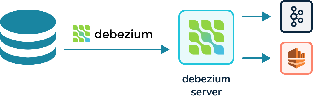
@@ -38,7 +38,7 @@ Capturing change events requires specific knowledge of the
database from which t
Kafka connectors must run in a Kafka Connect cluster, a highly available and
distributed system for running connectors. Kafka connectors cannot run on their
own and require a server. The Debezium project provides a Debezium server that
can also run Debezium connectors capable of writing to other event streaming
platforms besides Kafka, for instance, Amazon Kinesis. The diagram below shows
a Debezium connector reading the WAL and writing to a Debezium server. The
Debezium server can then [...]
-
+
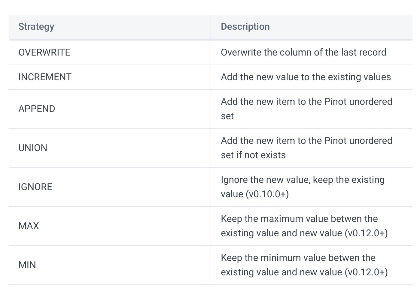
## Debezium Data Format
@@ -180,7 +180,7 @@ A FULL upsert means that a new record will replace the
older record completely i
PARTIAL only allows updates to specific columns and employs additional
strategies.
-
+
Source: [Stream Ingestion with
Upsert](https://docs.pinot.apache.org/basics/data-import/upsert)
diff --git
a/data/blog/2023-05-30-how-to-ingest-streaming-data-from-kafka-to-apache-pinot.mdx
b/data/blog/2023-05-30-how-to-ingest-streaming-data-from-kafka-to-apache-pinot.mdx
index a4de9825..2bfbc4b5 100644
---
a/data/blog/2023-05-30-how-to-ingest-streaming-data-from-kafka-to-apache-pinot.mdx
+++
b/data/blog/2023-05-30-how-to-ingest-streaming-data-from-kafka-to-apache-pinot.mdx
@@ -32,7 +32,7 @@ We will be installing Apache Kafka onto our already existing
Pinot docker image.
docker run -it --entrypoint /bin/bash -p 9000:9000
apachepinot.docker.scarf.sh/apachepinot/pinot:0.12.0
-
+
We want to override the ENTRYPOINT and run Bash script within the Docker
image. If you already have a container running, you can skip this step. I tend
to tear down containers after use, so in my case, I created a brand new
container.
@@ -54,11 +54,11 @@ Run each of the commands one at a time. The & allows you to
continue using the s
It should look like this:
-
+
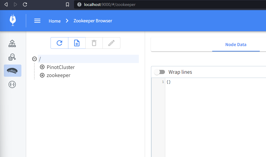
You can now browse to
[http://localhost:9000/#/zookeeper](http://localhost:9000/#/zookeeper) to see
the running cluster:
-
+
### Step 2: Install Kafka on the Docker container
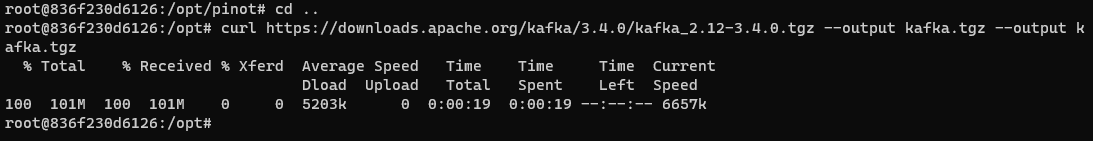
@@ -75,7 +75,7 @@ curl
https://downloads.apache.org/kafka/3.4.0/kafka_2.12-3.4.0.tgz --output kafk
It should look this:
-
+
Note that we’ve changed the directory to keep the Kafka folder separate from
the Pinot folder.
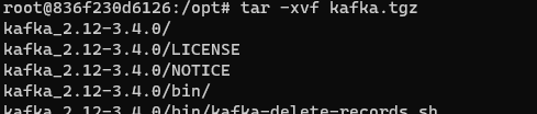
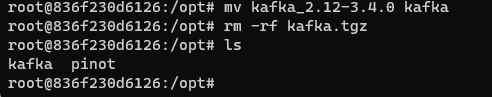
@@ -89,9 +89,9 @@ rm -rf kafka.tgz
It should look like this:
-
+
-
+
Now, Kafka and Pinot reside locally on our Docker container with Pinot up and
running. Let’s run the Kafka service. Kafka will use the existing ZooKeeper for
configuration management.
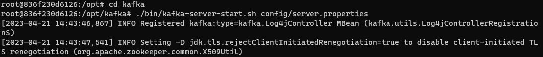
@@ -104,11 +104,11 @@ cd kafka
It should look like this:
-
+
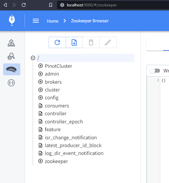
To verify that Kafka is running, let’s look at our ZooKeeper configs by
browsing to
[http://localhost:9000/#/zookeeper:](http://localhost:9000/#/zookeeper)
-
+
You may have to refresh the page and find many more configuration items appear
thanexpectedt. These are Kafka configurations.
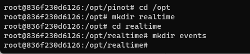
@@ -128,7 +128,7 @@ mkdir events
It should look like this:
-
+
You may have to start a new PowerShell window and connect to Docker for this.
Now, let’s install Node.js and any dependencies we might need for the event
consumption script:
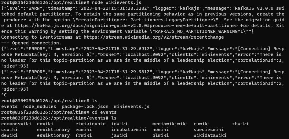
@@ -207,15 +207,15 @@ node wikievents.js
Use Ctrl-C to stop the program. Navigate to the events folder to see some new
folders created with the various language events downloaded from Wikipedia.
-
+
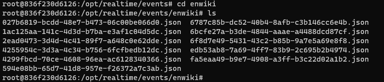
Navigate to the enwiki folder and review some of the downloaded JSON files.
-
+
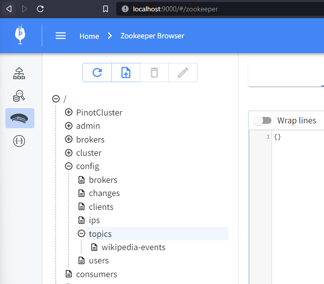
At http://localhost:9000/#/zookeeper, you can find the Kafka topic by locating
the ZooKeeper config and expanding config > topics. You may have to refresh
your browser.
-
+
Here, you should see the wikipedia-events topic that we created using the
Node.js script. So far, so good.
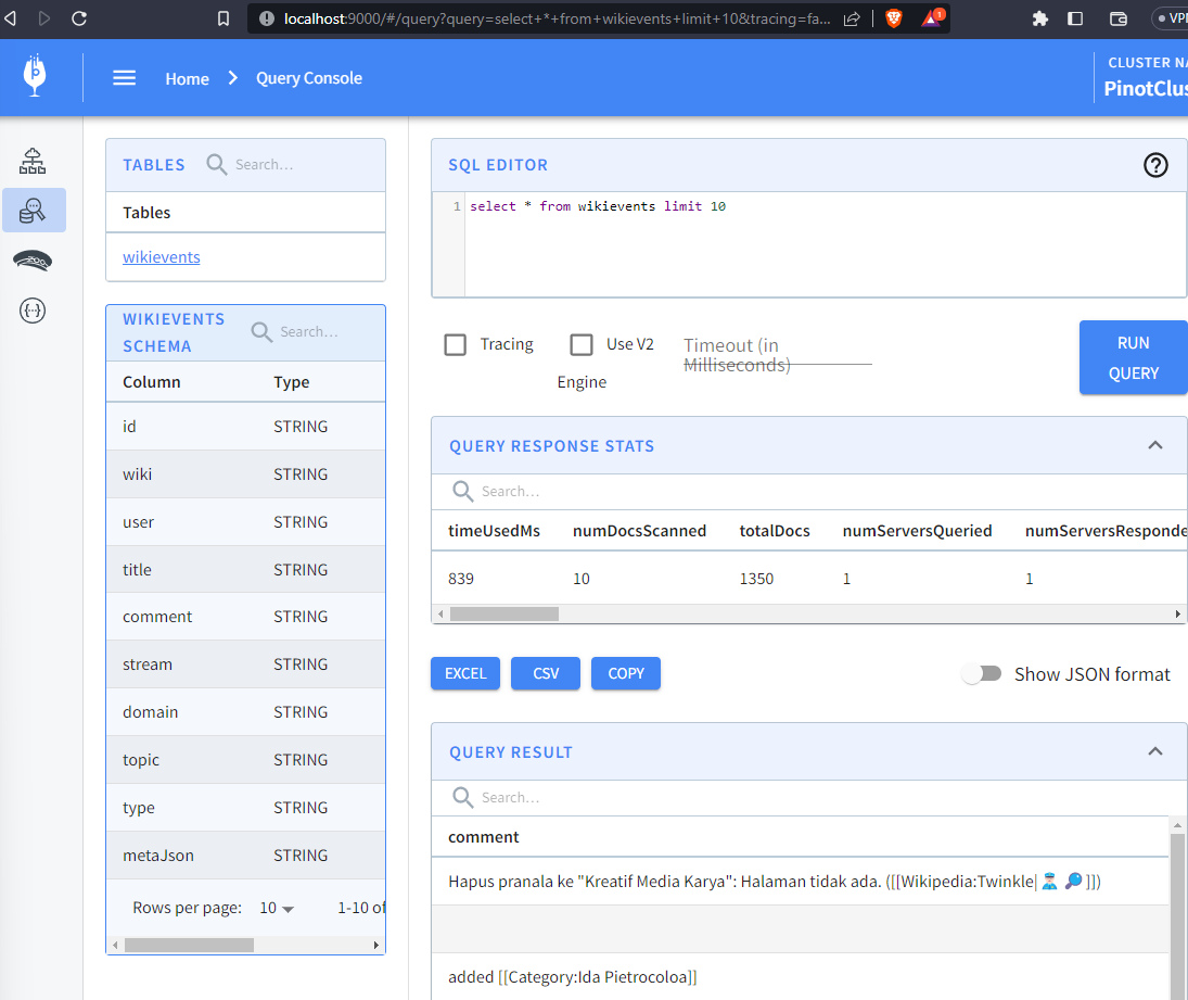
@@ -374,7 +374,7 @@ Now, browse to the following location
[http://localhost:9000/#/tables,](http://l
Run the node wikievents.js command, then query the newly created wikievents
table to see the totalDocs increase in real time:
-
+
To avoid running out of space on your computer, make sure to stop the
wikievents.js script when you’re done :-D
diff --git
a/data/blog/2023-06-01-real-time-mastodon-usage-with-apache-kafka-apache-pinot-and-streamlit.mdx
b/data/blog/2023-06-01-real-time-mastodon-usage-with-apache-kafka-apache-pinot-and-streamlit.mdx
index 3844f118..12b11d07 100644
---
a/data/blog/2023-06-01-real-time-mastodon-usage-with-apache-kafka-apache-pinot-and-streamlit.mdx
+++
b/data/blog/2023-06-01-real-time-mastodon-usage-with-apache-kafka-apache-pinot-and-streamlit.mdx
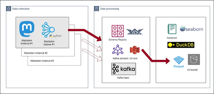
@@ -39,7 +39,7 @@ To start, Simon wrote a listener to collect the messages,
which he then publishe
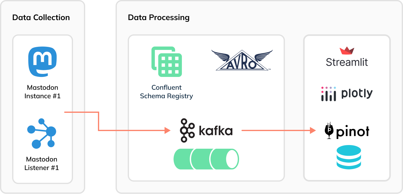
Finally, he queried those Parquet files using DuckDB and created some charts
using the Seaborn library, as reflected in the architecture diagram below:
-
+
Fig: [Data Collection
Architecture](https://simonaubury.com/posts/202302_mastodon_duckdb/)
@@ -49,7 +49,7 @@ The awesome visualizations that Simon created make me wonder
whether we can chan
Now [Apache Pinot](https://startree.ai/resources/what-is-apache-pinot) comes
into the picture. Instead of using Kafka Connect to batch Mastodon toots into
groups of 1,000 messages to generate Parquet files, we can stream the data
immediately and directly, toot-by-toot into Pinot and then build a real-time
dashboard using Streamlit:
-
+
## Setup
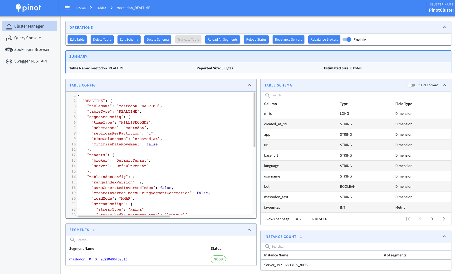
@@ -191,7 +191,7 @@ We can then navigate to the table page of the Pinot UI:
Here, we’ll see the following:
-
+
## Ingest Data into Kafka
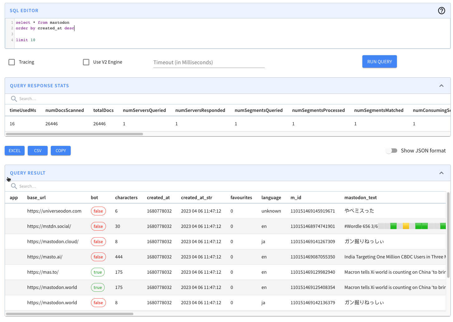
@@ -221,7 +221,7 @@ Now, let’s go to the Pinot UI to see what data we’ve got to
play with:
We’ll see the following preview of the data in the mastodon table:
-
+
We can then write a query to find the number of messages posted in the last
five minutes:
@@ -234,7 +234,7 @@ where created_at*1000 > ago('PT1M')
order by 1 DESC;
```
-
+
We can also query Pinot via the Python client, which we can install by running
the following:
@@ -283,19 +283,19 @@ I’ve created a Streamlit app in the file
[app.py](https://github.com/mneedham/
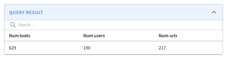
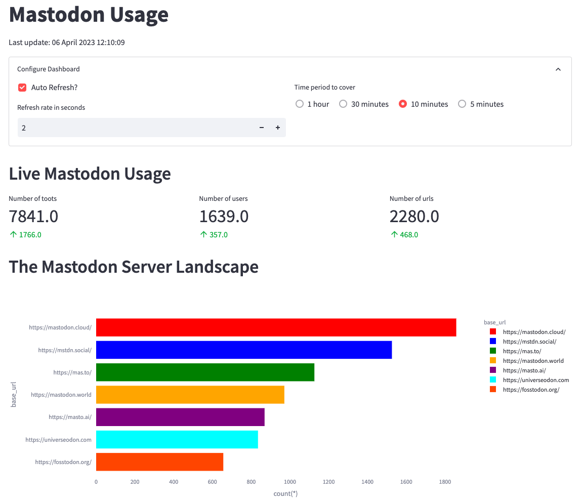
First, we’ll create metrics to show the number of toots, users, and URLs in
the last _n_ minutes. _n_ will be configurable from the app as shown in the
screenshot below:
-
+
From the screenshot, we can identify mastodon.cloud as the most active server,
though it produces only 1,800 messages in 10 minutes or three messages per
second. The values in green indicate the change in values compared to the
previous 10 minutes.
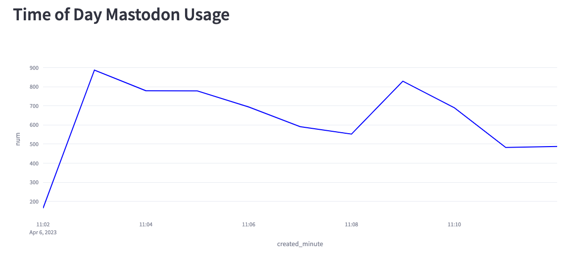
We can also create a chart showing the number of messages per minute for the
last 10 minutes:
-
+
Based on this chart, we can see that we’re creating anywhere from 200–900
messages per second. Part of the reason lies in the fact that the Mastodon
servers sometimes disconnect our listener, and at the moment, I have to
manually reconnect.
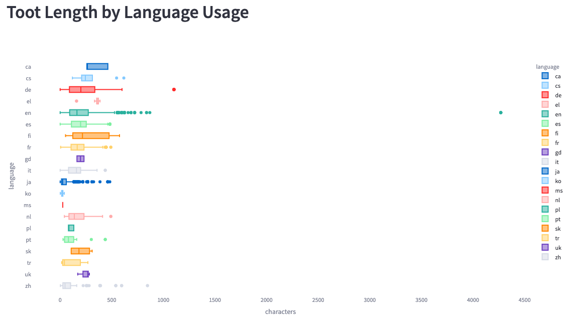
Finally, we can look at the toot length by language:
-
+
We see much bigger ranges here than Simon saw in his analysis. He saw a
maximum length of 200 characters, whereas we see some messages of up to 4,200
characters.
diff --git
a/data/blog/2023-07-12-star-tree-index-in-apache-pinot-part-3-understanding-the-impact-in-real-customer.mdx
b/data/blog/2023-07-12-star-tree-index-in-apache-pinot-part-3-understanding-the-impact-in-real-customer.mdx
index 679e2e5f..2a5328c7 100644
---
a/data/blog/2023-07-12-star-tree-index-in-apache-pinot-part-3-understanding-the-impact-in-real-customer.mdx
+++
b/data/blog/2023-07-12-star-tree-index-in-apache-pinot-part-3-understanding-the-impact-in-real-customer.mdx
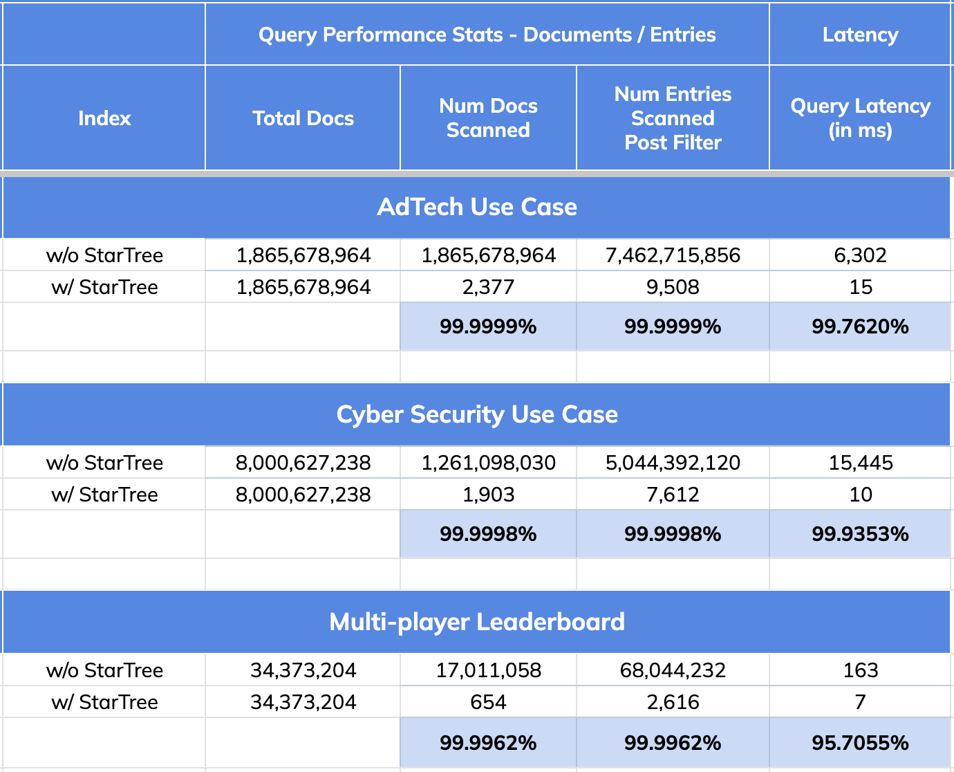
@@ -70,7 +70,7 @@ This is exactly the type of scenario that the [Star-Tree
Index](https://docs.pin
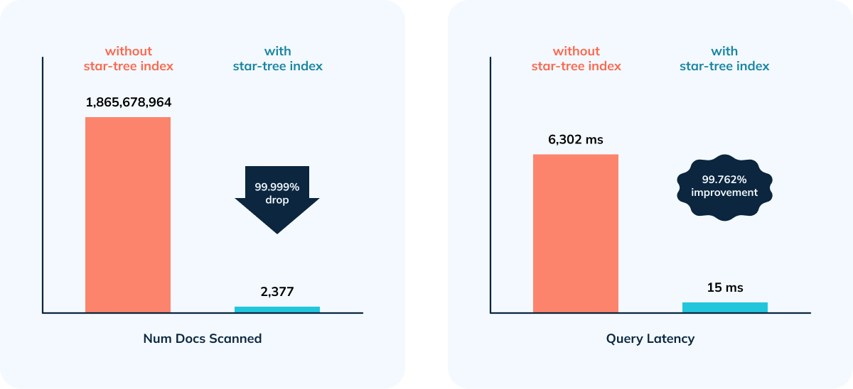
- 99.76% reduction in latency vs. no Star-Tree Index (6.3 seconds to 15 ms)
- 99.99999% reduction in amount of data scanned/aggregated per query (> 1.8B
docs to < 2,400)
-
+
## CyberSecurity Use Case:
@@ -105,7 +105,7 @@ Given the overhead while doing complex aggregations,
efficient filtering (indexe
- 99.9998% reduction in data scanned/aggregated per query
- Happy Customer 😃
-
+
## Multiplayer Game Leaderboard Use Case
@@ -131,11 +131,11 @@ Given the overhead while doing complex aggregations,
efficient filtering (indexe
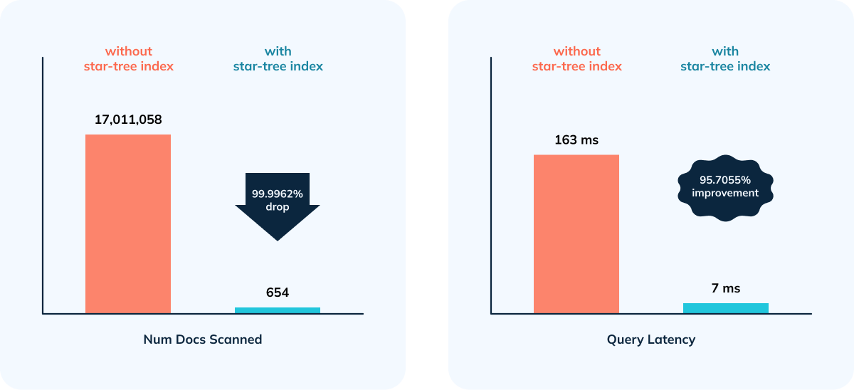
- 95.70% improvement in query performance as a result of 99.9962% reduction
in number of documents and entries scanned.
-
+
## Quick Recap: Star-Tree Index Performance Improvements
-
+
- 99.99% reduction in data scanned/aggregated per query
- 95 to 99% improvement in query performance
---------------------------------------------------------------------
To unsubscribe, e-mail: [email protected]
For additional commands, e-mail: [email protected]